R
Installing R
- Navigate to https://cran.r-project.org/mirrors.html.
- Choose a location near you under USA and click the hyperlink
- On this page, there are downloads available for each system. Click the link for your system.
- Click base
- Click the Download link at the top, Save File and proceed through the download and install.
GUI for R
We recommend installing a GUI for R, such as RStudio or Tinn-R. This will provide a nice interface for working with R.
ANOVA
One-Way
-
Create lists of the data (vectors) that you want to make an ANOVA for. In this case, the response variable (y) is the selling price (in thousands of dollars) and x represents the sales person who each sold 4 robots at y selling price. Note in this example that it is necessary to use strings for x instead of numbers. R reads these strings like humans read words. In other words, the number assigned to each salesperson is arbitrary and could be named anything. For instance, as humans we recognize that the problem would be comparable if we named the sales people "Rebecca", "Rachel", and "Raymond" instead of "1", "2", and "3" but R needs to be specifically told to read them as a string and not a number.
> SellingPrices <- c(10,14,13,12,11,16,14,15,11,13,12,15) greater than Selling Prices less than minus c left parenthesis ten, fourteen, thirteen, twelve, eleven, sixteen, fourteen, fifteen, eleven, thirteen, twelve, fifteen right parenthesis
> Salesperson <- c("1", "1", "1", "1", "2", "2", "2", "2", "3", "3", "3", "3") greater than Salesperson less than minus c left parenthesis One, One, One, One, Two, Two, Two, Two, Three, Three, Three, Three right parenthesis -
Next make a data frame for the variables which enables R to read them as one set of data instead of two independent columns.
> values = data.frame(SellingPrices, Salesperson)greater than values equals data frame left parenthesis Selling Prices, Sales Person right parenthesis
> summary(values)greater than summary left parenthesis values right parenthesis## SellingPrices Salesperson ## Min. :10.00 1:4 ## 1st Qu.:11.75 2:4 ## Median :13.00 3:4 ## Mean :13.00 ## 3rd Qu.:14.25 ## Max. :16.00 -
Use the aov(y ~ x, data = data frame) to run a one-way ANOVA. Then use the summary() function to look up key outputs from the ANOVA.
> SellingPrice.aov <- aov (SellingPrices ~ Salesperson, data = values)greater than Selling Price aov less than minus aov left parenthesis Selling Prices tilde Sales person, data equals values right parenthesis
> summary(SellingPrice.aov)greater than summary left parenthesis Selling Price aov right parenthesis## Df Sum Sq Mean Sq F value Pr(>F) ## Salesperson 2 6.5 3.25 0.929 0.43 ## Residuals 9 31.5 3.50
Read more about making your own ANOVAs here.
Binomial Distribution
Binomial Probability (pdf)
-
Into the console type dbinom(successes, number of trials, probability of success)dbinom left parenthesis successes, number of trials, probability of success right parenthesis. The result is shown in row [1].
> dbinom(0, 4, 1/6)greater than dbinom left parenthesis zero, four, one divided by six right parenthesis
[1] 0.4822530864
Binomial Probability Distribution
-
Into the console type dbinom(successes, number of trials, probability of success). The result is shown in row [1].
> dbinom(0:4, 4, 1/6)greater than dbinom left parenthesis zero colon four, four, one divided by six right parenthesis
[1] 0.4822530864 0.3858024691 0.1157407407 0.0154320988 0.0007716049
Note: Here we have entered 0:4zero colon four for successes to calculate the entire distribution at once. The first probability (0.4822530864zero point four eight two two five three zero eight six four) in the output corresponds to 0 successes, the second (0.4822530864zero point four eight two two five three zero eight six four) corresponds to 1 success, and so on. Individual probabilities can be found by instead entering a single number here, such as "dbinom(0, 4, 1/6)dbinom left parenthesis zero, four, One divided by six right parenthesis".
Binomial Probability (cdf)
-
Into the console type pbinom(successes, number of trials, probability of success)pbinom left parenthesis successes, number of trials, probability of success right parenthesis. The result is shown in row [1].
> pbinom(11,20,0.4)greater than pbinom left parenthesis Eleven, Twenty, zero point four right parenthesis
[1] 0.9434736
Chi-Square Distribution
Critical Value
-
Into the console type "qchisq(1-a, degrees of freedom)qchisq left parenthesis 1 minus alpha, degrees of freedom right parenthesis". The chi-square critical value corresponding to probability a in the right tail is returned. The result is shown in row [1].
> qchisq(.99,13)greater than qchisq left parenthesis point Nine nine, 13 right parenthesis
[1] 27.68825
Left Tailed Probability (cdf)
To find the corresponding p-value for a left tailed probability (cdf) X2 test statistic, use pchisq(x, degrees of freedom, lower.tail = TRUE)pchisq left parenthesis x, degrees of freedom, lower tail equals True right parenthesis.
> pchisq(120,2,lower.tail = TRUE)greater than pchisq left parenthesis one hundred twenty, two lower tail equals True right parenthesis
## [1] 1
Read more about chi-square distribution probability distributions here.
Right Tailed Probability (cdf)
To find the corresponding p-value for a right tailed probability (cdf) X2 test statistic, use pchisq(x, degrees of freedom, lower.tail = FALSE)pchisq left parenthesis x, degrees of freedom, lower tail equals False right parenthesis.
> pchisq(120,2,lower.tail = FALSE)greater than pchisq left parenthesis one hundred twenty, two, lower tail equals False right parenthesis
## [1] 8.756511e-27
Read more about chi-square distribution probability distributions here.
Confidence Intervals
Proportion
-
To make a proportion confidence interval you will use the binom.test(x,n)binom test left parenthesis x, n right parenthesis function. You will need to enter the following parameters into the function: x being the number of cases, n being the total sample size. Example: You take a sample of 10 people. 5 of them are female. Confidence level defaults to 95%
-
You can change the confidence level using the parameter conf.levelformula conf level.
> binom.test(5,10)greater than binom test left parenthesis five, ten right parenthesis
Exact binomial test
data: 5 and 10
number of successes = 5, number of trials = 10, p-value = 1
alternative hypothesis: true probability of success is not equal to 0.5
95 percent confidence interval:
0.187086 0.812914
sample estimates:
probability of success
0.5
> binom.test(5,10,conf.level=.90)greater than binom test left parenthesis five, ten, conf level equals point nine zero right parenthesis
Exact binomial test
data: 5 and 10
number of successes = 5, number of trials = 10, p-value = 1
alternative hypothesis: true probability of success is not equal to 0.5
90 percent confidence interval:
0.2224411 0.7775589
sample estimates:
probability of success
0.5
t-Interval
-
To make a t-interval you will need your data saved in an array.
-
You can perform the t-interval calculation using the function t.test()t test left parenthesis right parenthesis. The function will automatically calculate the necessary sample statistics. Confidence level defaults to 95%.
-
You can change the confidence level using the parameter conf.levelformula conf level.
> age=c(24,25,27,33,35,37)greater than age equals c left parenthesis twenty four, twenty five, twenty seven, Thirty three, Thirty five, Thirty seven right parenthesis
> t.test(age)greater than t test left parenthesis age right parenthesis
One Sample t-test
data: age
t = 13.365, df = 5, p-value = 4.195e-05
alternative hypothesis: true mean is not equal to 0
95 percent confidence interval:
24.36464 35.96870
sample estimates:
mean of x
30.16667
> t.test(age,conf.level=.90)greater than t test left parenthesis age, conf level equals poinr Nine zero right parenthesis
One Sample t-test
data: age
t = 13.365, df = 5, p-value = 4.195e-05
alternative hypothesis: true mean is not equal to 0
90 percent confidence interval:
25.61853 34.71481
sample estimates:
mean of x
30.16667
z-Interval
To make a z-interval you will use R to make the calculation by hand
-
To make a z-interval you will need your data saved in an array.
-
Save the following parameters in a variable.
-
Sample mean
-
Sample standard deviation
-
Sample size
-
-
Now you need to determine the Critical Value to use using the qnorm()qnorm left parenthesis right parenthesis function. Decide on your Confidence Level. The typical options are 90%, 95%, or 99%. Subtract that percentage from 100%, cut in half, and convert to a decimal to use in the qnorm() function. For Example: For a 95% confidence interval, take half of 5% or 2.5% (.025).
-
Calculate the Margin of Error by multiplying the critical value times standard deviation, then dividing by square root of sample size.
-
Calculate the confidence interval by adding and subtracting the margin of error from the sample mean.
> age=c(24,25,27,33,35,37)greater than age equals c left parenthesis Twenty four, Twenty five, Twenty seven, Thirty three, Thirty five, thirty seven right parenthesis
> mean=mean(age)greater than mean equals mean left parenthesis age right parenthesis
> sd=sd(age)greater than sd equals sd left parenthesis age right parenthesis
> n=length(age)greater than n equals length left parenthesis age right parenthesis
> z=qnorm(.025)greater than z equals qnorm left parenthesis point zero two five right parenthesis
> zgreater than z
[1] -1.959964
> MOE=z*sd/sqrt(n)greater than MOE equals z asterisk times sd divided by sqrt left parenthesis n right parenthesis
> mean-MOEgreater than mean minus MOE
[1] 34.59048
> mean+MOEgreater than mean plus MOE
[1] 25.74286
Two Sample t-Interval (Independent Samples)
-
To make a Two Sample t-interval you will need each sample's data saved in a separate array.
-
You can perform the t-interval calculation using the function t.test()t test left parenthesis right parenthesis. The function will automatically calculate the necessary sample statistics. Confidence level defaults to 95%.
-
You can change the confidence level using the parameter conf.levelconf level.
> agemen=c(24,25,27,33,35,37)greater than agemen equals c left parenthesis twenty four, twenty five, twenty seven, Thirty three, Thirty five, Thirty seven right parenthesis
> agewomen=c(24,34,22,18,33,25)greater than agewomen equals c left parenthesis twenty four, Thirty four, Twenty two, Eighteen, Thirty three, twenty five right parenthesis
> t.test(agemen,agewomen)greater than t test left parenthesis agemen, agewomen right parenthesis
Welch Two Sample t-test
data: agemen and agewomen
t = 1.2184, df = 9.837, p-value = 0.2515
alternative hypothesis: true difference in means is not equal to 0
95 percent confidence interval:
-3.470084 11.803418
sample estimates:
mean of x mean of y
30.16667 26.00000
> t.test(agemen,agewomen,conf.level=.90)greater than t test left parenthesis agemen, agewomen, conf level equals point nine zero right parenthesis
Welch Two Sample t-test
data: agemen and agewomen
t = 1.2184, df = 9.837, p-value = 0.2515
alternative hypothesis: true difference in means is not equal to 0
90 percent confidence interval:
-2.041873 10.375206
sample estimates:
mean of x mean of y
30.16667 26.00000
Two Sample z-Interval
To make a two sample z-interval you will use R to make the calculation by hand.
-
To make a two sample z-interval you will need each sample's data saved in a separate array.
-
Sample mean 1 and 2
-
Sample variance 1 and 2
-
Sample size 1 and 2
-
-
Now you need to determine the Critical Value to use using the qnorm()qnorm left parenthesis right parenthesis function. Decide on your Confidence Level. The typical options are 90%, 95%, or 99%. Subtract that percentage from 100%, cut in half, and convert to a decimal to use in the qnorm()qnorm left parenthesis right parenthesis function. For Example: For a 95% confidence interval, take half of 5% or 2.5% (.025).
-
Calculate the Margin of Error by multiplying the critical value times the square root of the sum of each variance divided by its sample size.
-
Calculate the sample difference by subtracting the two sample means.
-
Calculate the confidence interval by adding and subtracting the margin of error from the sample difference.
> agemen=c(24,25,27,33,35,37)greater than agemen equals c left parenthesis twenty four, twenty five, twenty seven, Thirty three, Thirty five, Thirty seven right parenthesis
> agewomen=c(24,34,22,18,33,25)greater than agewomen equals c left parenthesis twenty four, Thirty four, Twenty two, Eighteen, Thirty three, twenty five right parenthesis
> meanM=mean(agemen)greater than meanM equals mean left parenthesis agemen right parenthesis
> meanW=mean(agewomen)greater than meanW equals mean left parenthesis agewomen right parenthesis
> varM=var(agemen)greater than varM equals var left parenthesis agemen right parenthesis
> varW=var(agewomen)greater than varW equals var left parenthesis agewomen right parenthesis
> nM=length(agemen)greater than nM equals length left parenthesis agemen right parenthesis
> nW=length(agewomen)greater than nW equals length left parenthesis agewomen right parenthesis
> z=qnorm(.025)greater than z equals qnorm left parenthesis point zero two five right parenthesis
> zgreater than z
[1] -1.959964
> MOE=z*sqrt(varM/nM+varW/nW)greater than MOE equals z asterisk times sqrt left parenthesis varM divided by nM plus varW divided by nW right parenthesis
> diff=meanM-meanWgreater than diff equals meanM minus meanW
> diff-MOEgreater than diff minus MOE
[1] 10.86918
> diff+MOEgreater than diff plus MOE
[1] -2.53585
Counting
Combination
The number of combinations can found by using combncombn. Input the number of objects first (36) followed by the number of objects taken at a time (5). The ncol command counts the number of combinations in this case.
> ncol(combn(36,5)greater than ncol left parenthesis combn left parenthesis Thirty six, five right parenthesis
## [1] 376992
Read more about programming your combinations here.
Factorial
Use the factorial()factorial left parenthesis right parenthesis function to find the factorial.
> factorial(5)greater than factorial left parenthesis 5 right parenthesis
## [1] 120
Read more about how to use the factorial function here.
Permutation
Since there is no simple command for a permutation like there is for combinations, it is easiest to calculate a permutation by using what we know about combinations. Permutations are simply a combination multiplied by k! or the factorial of the number selected at a time. Without using the number of columns function (ncolncol), we would receive a list of all permutations.
> ncol(combn(7,3))*factorial(3)greater than ncol left parenthesis combn left parenthesis seven, three right parenthesis right parenthesis asterisk times factorial left parenthesis three right parenthesis
## [1] 210
Data Manipulation
Sorting
To sort data by ascending or descending order, use the sort()sort left parenthesis right parenthesisfunction. In this example, we will sort the ages of 25 employees at a clothing department store (Example 3.4.2).
-
Create a list of all the ages to be included. This list (or vector) is called "Ages" here. Alternatively, you could extract a column or row of data from an Excel to sort it.
> Ages <-c(32,21,24,19,61,18,18,16,16,35,39,17,22,21,60,18,53,18,57,63,28,20,29,35,45)greater than Ages less than minus c left parenthesis Thirty two, Twenty one, Twenty four, Nineteen, Sixty one, Eighteen, Eighteen, Sixteen, Sixteen, Thirty five, Thirty nine, Seventeen, Twenty two, Twenty one, Sixty, Eighteen, Fifty three, Eighteen, Fifty seven, Sixty three, Twenty eight, Twenty, Twenty Nine, Thirty five, Fourty five right parenthesis
-
Use sort(x, decreasing=FALSE)sort left parenthesis x, decreasing equals False right parenthesis to sort in ascending order (smallest to largest). Set decreasing=TRUEdecreasing equals True for descending order (largest to smallest).
> sort(Ages, decreasing=FALSE)greater than sort left parenthesis Ages, decreasing equals False right parenthesis
## [1] 16 16 17 18 18 18 18 19 20 21 21 22 24 28 29 32 35 35 39 45 53 57 60
## [24] 61 63
Read more about sorting your data here.
Descriptive Statistics
One Variable
There are a variety of functions and packages that can be used to calculate descriptive statistics. In addition to the base functions in R, packages such as "mosaic" can be used to calculate descriptive statistics.
> list <- c(4,10,7,15)greater than list less than minus c left parenthesis four, ten, seven, fifteen right parenthesis
One of the easiest ways to see the mean, median, maximum, and minimum of a data set is to use the summary() function. Note that there is no simple function to find the mode of a data set.
> summary(list)greater than summary left parenthesis list right parenthesis
| ## | Min. | 1st Qu. | Median | Mean | 3rd Qu. | Max. |
| ## | 4.00 | 6.25 | 8.50 | 9.00 | 11.25 | 15.00 |
The standard deviation, stadard error, variation, range, and sum can also be calculated easily.
> se <- sd(list)/sqrt(length(list))greater than se less than minus sd left parenthesis list right parenthesis divided by sqrt left parenthesis length left parenthesis list right parenthesis right parenthesis#Standard error calculation which is the standard deviation divided by the squareroot of the list's lengthhash Standard error calculation which is the standard deviation divided by the squareroot of the list apostrophe's length
> segreater than se
## [1] 2.345208
> sd(list)greater than sd left parenthesis list right parenthesis #Standard deviation functionhash Standard deviation function
## [1] 4.690416
> var(list)greater than var left parenthesis list right parenthesis#Variance functionhash Variance function
## [1] 22
> range.value <- (max(list)-min(list))greater than range value less than minus left parenthesis max left parenthesis list right parenthesis minus min left parenthesis list right parenthesis right parenthesis #Calculation for range which is the maximum value minus the minimum valuehash Calculation for range which is the minimum value
## [1] 11
> sum(list)greater than sum left parenthesis list right parenthesis #Sum of the valueshash Sum of the values
## [1] 36
Alternatively, you can install the "mosaic" package in R to use the favstats function. This will show you data on the minimum, maximum, mean, median, standard deviation, and count amoung other basic descriptors.
> install.packages("mosaic")greater than install.packages left parenthesis mosaic right parenthesis
> library("mosaic")greater than library left parenthesis mosaic right parenthesis
> favstats(list)greater than favstats left parenthesis list right parenthesis
| ## | min. | Q1 | median | Q3 | max | mean | sd | n | missing |
| ## | 4 | 6.25 | 8.5 | 11.25 | 15 | 9 | 4.690416 | 4 | 0 |
F-Distribution > F-Probability (cdf)
F-Probability (cdf)
Once you find the test statistic F and the degrees of freedom, then you can plug your values into the function to find the P-value.
F-statistic: 0.9286
Degrees of freedom: 2,9
P(F>0.9286): lower.tail=FALSE
> pf(0.9286,2,9,lower.tail=FALSE)greater than pf left parenthesis zero point nine two eight six, two, nine, lower tail equals FALSE right parenthesis
## [1] 0.4298936
Read more about F-Probability (cdf) here.
Graphs
Bar Charts
-
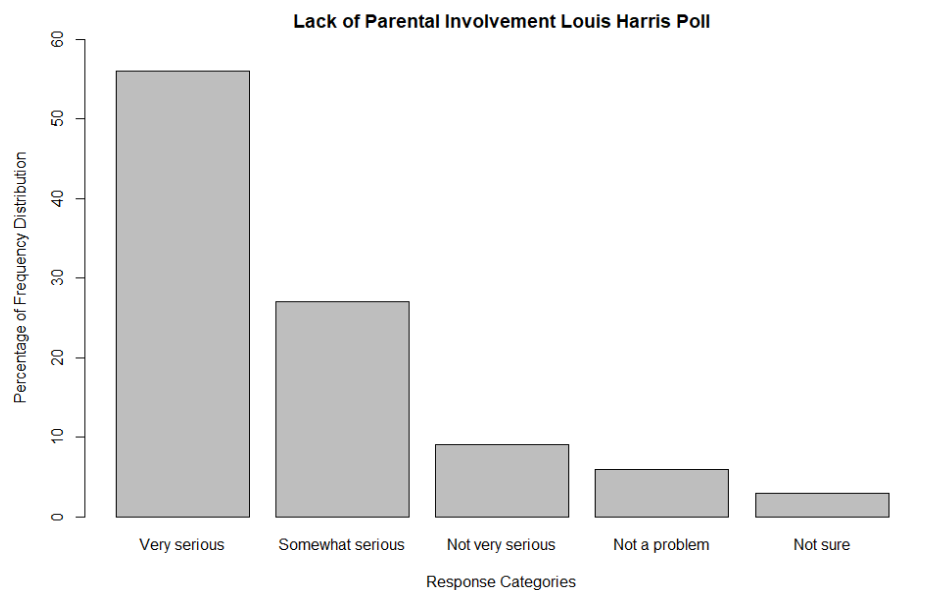
Create vectors (lines of your data) for x and y. Here, x is the Lack of Parental Involvement and y is the Percentage of Frequency Distribution for the responses.
aaaaaaaaaaa class="formula" aria-hidden="true">Lack_of_Parental_Involvement <- c(Very serious, Somewhat serious, Not very serious, Not a problem, Not sure)Lack underscore of underscore Parental underscore Involvement less than minus c left parenthesis Very serious, Somewhat serious, Not very serious, Not a problem, Not sure right parenthesis
> Percents <- c(56,27,9,6,3)greater than Percents less than minus c left parenthesis fifty six, twenty seven, nine, six, three right parenthesis -
Plot the bar chart using barplot()barplot left parenthesis right parenthesis.Percents acts as the height of the bar chart and the names for the widths of the bars are represented by the responses for Lack of Parental Involvement. xlabxlab and ylabylabylimylim is used to show the distribution of response percentage from 0-60%.
> barplot(Percents, names.arg=Lack_of_Parental_Involvement,main="Lack of Parental Involvement Louis Harris Poll", xlab="Response Categories", ylab="Percentage of Frequency Distribution", ylim=c(0,60)) greater than barplot left parenthesis Percents, names arg equals Lack underscore of underscore Parental underscore Involvement, main equals Lack of Parental Involvement Louis Harris Poll, xlab equals Response Categories , ylab equals Percentage of Frequency Distribution, ylim equals c left parenthesis zero, sixty right parenthesis right parenthesis
Read more about bar charts here.
Box Plots
-
Write your data as a list of numbers (vectors). For this example, the highest and lowest 5 wins per seasons were included from the Braves, Cubs, Dodgers, and Yankees baseball teams from the years 1967-2010.
> Bravesgreater than Braves <- c(50,54,61,63,65,106,104,103,101,101)less than minus c left parenthesis fifty, fifty four, sixty one, sixty three, sixty five, one hundred six, one hundred four, one hundred three, one hundred one, one hundred one right parenthesis
> Cubsgreater than Cubs <- c(38,49,61,64,65,103,97,97,96,93)less than minus c left parenthesis thirty eight, fourty nine, sixty one, sixty foru, sixty five, one hundred three, ninety seven, ninety seven, ninety six, ninety three right parenthesis
> Dodgersgreater than Dodgers <- c(58,63,63,71,73,102,98,95,95,95)less than minus c left parenthesis fifty eight, sixty three, sixty three, seventy one, seventy three, one hundred two, ninety eight, ninety five, ninety five, ninety five right parenthesis
> Yankeesgreater than Yankees <- c(59,67,70,71,72,114,103,103,103,101)less than minus c left parenthesis fifty nine, sixty seven, seventy, seventy one, seventy two, one hundred fourteen, one hundred three, one hundred three, one hundred three, one hundred one right parenthesis
-
For a boxplot with multiple columns, it is necessary to create a data frame which puts each data list as a column with 10 rows.
> BaseballTeamsgreater than BaseballTeams <- data.frame(Braves,Cubs,Dodgers,Yankees)less than minus data frame left parenthesis Braves, Cubs, Dodgers, Yankees right parenthesis
> BaseballTeamsgreater than BaseballTeams## Braves Cubs Dodgers Yankees ## 1 50 38 58 59 ## 2 54 49 63 67 ## 3 61 61 63 70 ## 4 63 64 71 71 ## 5 65 65 73 72 ## 6 106 103 102 114 ## 7 104 97 98 103 ## 8 103 97 95 103 ## 9 101 96 95 103 ## 10 101 93 95 101 -
Plot the boxplot using the data frame and appropriate labels.
> boxplotgreater than boxplot(BaseballTeams,ylim=c(35,120)greater than ylim equals c left parenthesis thirty five, one hundred twenty right parenthesis,xlab=xlab equals "Baseball Team"Baseball Team,ylab=formula r-input greater than ylab equals"Wins per Season"Wins per Season,main=greater than main equals"Box Plot of the Number of Franchise Wins per Season 1967-2010"Box Plot of the Number of Franchise Wins per Season 1967 minus 2010,col=cformula r minus input greater than col equals c("blue","yellow","red","green"blue, yellow, red, green),cex.main=.8formula r minus input greater than cex main equals point eight)

Read more about making your own boxplots here.
Choropleth Map (County)
-
Open RStudio.
-
Create a new project by clicking "FileFile" at the top of the window, and then selecting "New ProjectNew Project".
-
In the pop-up window, click "New DirectoryNew Directory" and then "Empty ProjectEmpty Project". Name it "Choropleth MapChoropleth Map", and save it wherever you prefer.
-
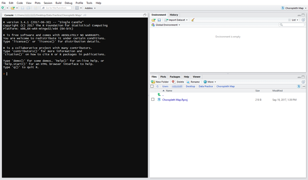
Upon creating your project, a section of your screen will show up with some text on it. Below the text there will be a ">greater than" symbol and the cursor should show up to the right of the symbol. This is called the R console, and this is where we will write our statements.
-
First, we will install all the necessary packages needed to create a choropleth map. Enter the following statements in the R console, pressing ENTERthe Enter key after each statement.
> install.packages("choroplethr")greater than install packages left parenthesis choroplethr right parenthesis
> install.packages("choroplethrMaps")greater than install packages left parenthesis choroplethr Maps right parenthesis
> library("choroplethr")greater than library left parenthesis choroplethr right parenthesis
> library("choroplethrMaps")greater than library left parenthesis choroplethr Maps right parenthesis
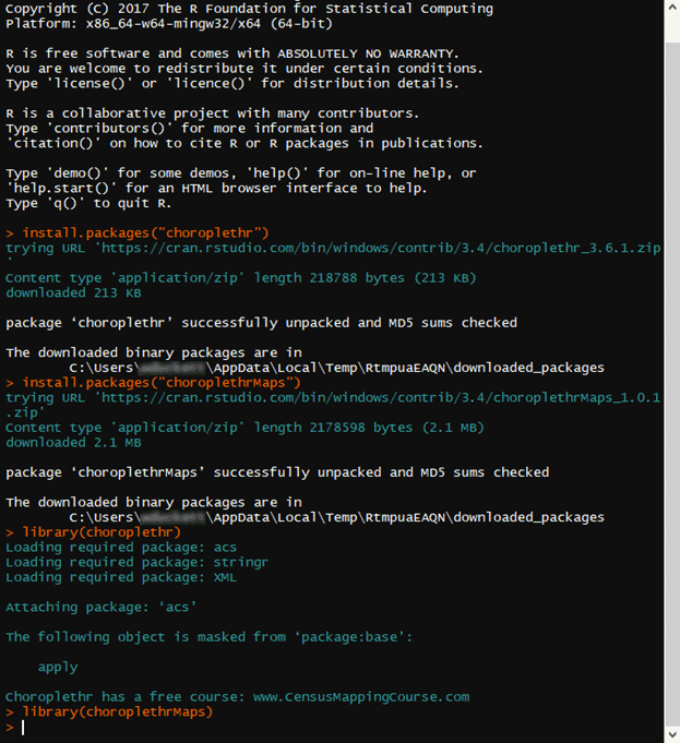
Note: the install.packages()install packages left parenthesis right parenthesis statements only need to be run once and the specified package will be installed permanently. However, installing a package is different from loading a package into R. We need to load packages into R using the library()library left parenthesis right parenthesis function every time we open a new R session.
-
Now that we have all of the necessary tools installed and loaded, it is time to load in our data. For county level data, the choropleth map package in R requires data to be in comma separated value format (.csv) and organized in the following way:
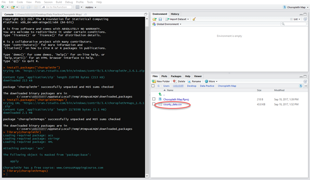
A B 1 region value 2 1001 8437 3 1003 39710 4 1005 2354 5 1007 1664 6 1009 5080 7 1011 1031 8 1013 2032 9 1015 13818 10 1017 2759 The first column must have a header titled "region" containing the geographic indicator (FIPS/county codes), and the second column must have a header titled "value" that contains the value of the variable of interest associated with the geographic indicator. Make sure that there is no extra formatting in either column (no commas, symbols, text, etc.) Save the correctly formatted .csv file in the same location that you created your new R project directory. You should see the file name appear in the "Files" pane.
For this example, we will use the US County Data found on the web resource.
-
Once the .csv is saved in the correct location, we can load it into R via the R console. Navigate to the console, type in the following statement, and press ENTERthe Enter key.
> mapData <- read.csv("county_data.csv")greater than map data less than minus read csv left parenthesis county underscore data csv right parenthesis
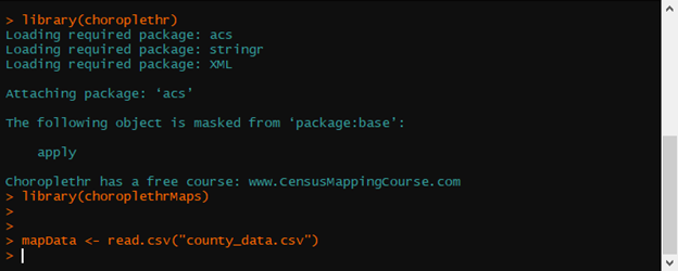
Note: The "<-less than minus" symbol denotes assignment. We are assigning the data from the .csv file to a variable named "mapData" so that we can easily access it for future use.
-
Once loaded, you should see an item in the Data panel with the name "mapData". By clicking on the item in the data panel, we can view the data that was loaded into R. The data should only have 2 variables (region, value). Now, we will create the choropleth map using a single R statement. Type the following into the console and press ENTERthe Enter key.
> county_choropleth(mapData)greater than county underscore choropleth left parenthesis map data right parenthesis
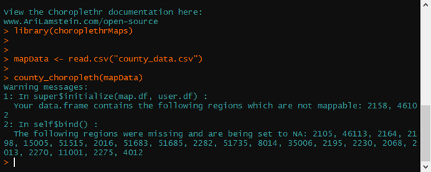
Depending on which FIPS codes are/aren't included in your dataset, you may get a warning message, but if there are no actual errors, the graph should still be generated like the following.
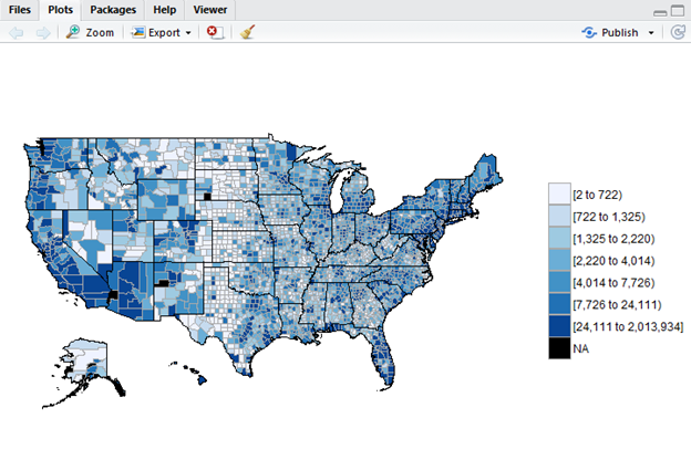
-
After a couple seconds, R will generate a map of the United States with the county regions shaded depending on the associated value. You can specify a title for the maps, and a title for the legend by typing the statement with some additional input or parameters.
> county_choropleth(mapData, title = "Number of Residents with a Bachelor's Degree or Higher, 2011-2015", legend = "Number of Residents with Degree")greater than county underscore choropleth left parenthesis map data, title equals number of Residents with a Bachelor apostrophe's degree or Higher, 2011 to 2015 legend equals number of residents with degree right parenthesis
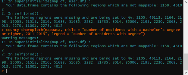
The previous command will generate the following plot.
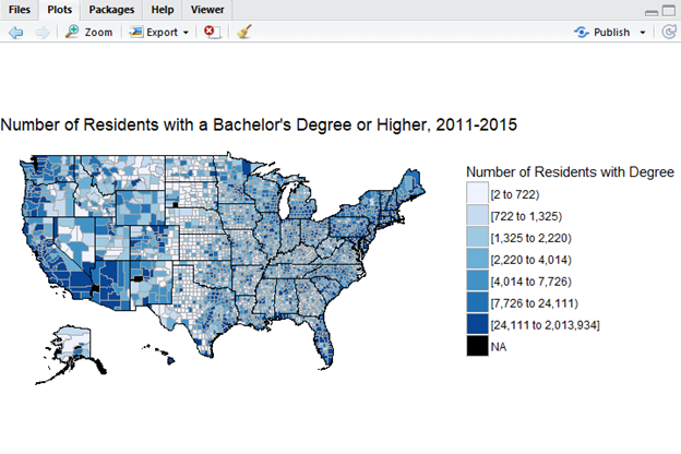
The plot can be saved as an image by clicking the "ExportExport" button above the graph and selecting "Save as Image…Save as Image horizontal ellipsis"
Histogram
-
Create a list of values (a vector) for your histogram. In this case, we are using the heart rate of 50 students.
> HeartRategreater than Heart Rate <-less than minus
c(77,84,79,90,67,84,82,74,88,75,69,81,94,68,65,86,78,79,79,70,83,83,84,82,93,80,81,80,87,80,62,98,77,83,82,80,82,73,85,77,77,79,81,70,72,85,84,80,74,83)c left parenthesis seventy seven, Eighty four, seventy nine, Ninety, sixty seven, Eighty four, Eighty two, seventy four, Eighty eight, seventy five, sixty nine, eighty one, ninety four, sixty eight, sixty five, eighty six,seventy eight, seventy nine, seventy nine, seventy, eighty three, eighty three, eighty four, eighty two, ninety three, eighty, eighty one, eighty, eighty seven, eighty, sixty two, ninety eight, seventy seven, eighty three, eighty two, eighty, eighty two, seventy three, eighty five, seventy seven, seventy seven, seventy nine, eighty one, seventy, seventy two, eighty five, eighty four, eighty, seventy four, eighty three right parenthesis -
Create a histogram with breaks using the number at the beginning of the interval (56.5 is an example here). This can be accomplished by using hist(). To create a histogram where the frequency of values is on the y-axis, make sure that the interval breaks are equally spaced.
> hist(HeartRate, breaks=c(56.5,66.5,76.5,86.5,96.5,106.5), main="Histogram of Heart Rates (per min.) of 50 Students", xlab= "Heart Rates (per min.)") greater than hist left parenthesis HeartRate, breaks equals c left parenthesis fifty six point five, sixty six point five, seventy six point five, eighty six point five, ninety six point five, one hundred six point five right parenthesis, main equals Histogram of Heart Rates left parenthesis per min right parenthesis of fifty Students, xlab equals Heart Rates left parenthesis per min right parenthesis right parenthesis

Read more about making your own histograms here.
Normal Probability Plot
-
Define your data variable by loading a datafile or entering a set of single variable data as a vector (in this case the data set was small so we defined it by hand).
-
Then, use qqnormqqnorm and qqlineqqline to create the plot and draw the trendline.
> exampleData <-c(20, 32, 14, 23, 27, 23, 29, 24, 23, 19)greater than example Data less than minus c left parenthesis twenty, thirty two, fourteen, twenty three, twenty seven, twenty three, twenty nine, twenty four, twenty three, nineteen right parenthesis
> qqnorm(exampleData, datax=TRUE)greater than qqnorm left parenthesis example Data, datax equals True right parenthesis
> qqline(exampleData, datax=TRUE)greater than qqline left parenthesis example Data, datax equals True right parenthesis
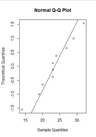
Note: If you left off ", datax=TRUE, datax equals True" the plot would be drawn with the sample quantities on the y-axis instead. Our materials typically show the data on the x-axis so we have adjusted this argument, but regardless of which axis has the data, you are looking for the points to follow a line.
Scatterplot
-
For this example, we are using the High School Completion and Crime Rate data from Hawkes Stat. Delete the title (High School Completion and Crime Rate 2014) of the dataset from the top while saving it to your computer.
-
Upload the data set to R. To do this, type in the name you want to save the data set as (in this case school_and_crime). To read the data into R, use read.csv(file="",header=TRUE,sep=","). Inside the "" you should put the path name to the file. You should then be able to view your data set in the Global Environment. More information about doing this can be found here.
> school_and_crime <- read.csv(file="", header=TRUE, sep=",") greater than school underscore and underscore crime less than minus read csv left parenthesis file equals open parenthesis close parenthesis, header equals True, sep equals , right parenthesis
-
Next you can plot your data. The $ are used to call a particular column of data from your file. In this case, the Crime Rate Data column is read as Crime.Rate..per.100.000 by R and the High School Completion column is read by R as High.School.Completion. Finally, label your axes and title.
plot(school_and_crime$Crime.Rate..per.100.000,school_and_crime$High.School.Completion, xlab="Crime Rate (per 100,000)", ylab="Completion Rate",main="High School Completion Rate and Crime Rate",ylim=c(65,95)) plotleft parenthesis school underscore and underscore crime dollar Crime Rate.. per one hundred, school underscore and underscore crime dollar High School Completion, xlab equalsCrime Rate left parenthesis per one lakh right parenthesis ylab equals Completion Rate, main equals"High School Completion Rate and Crime Rateylim equals c left parenthesissixty five, Ninety five right parenthesis right parenthesis
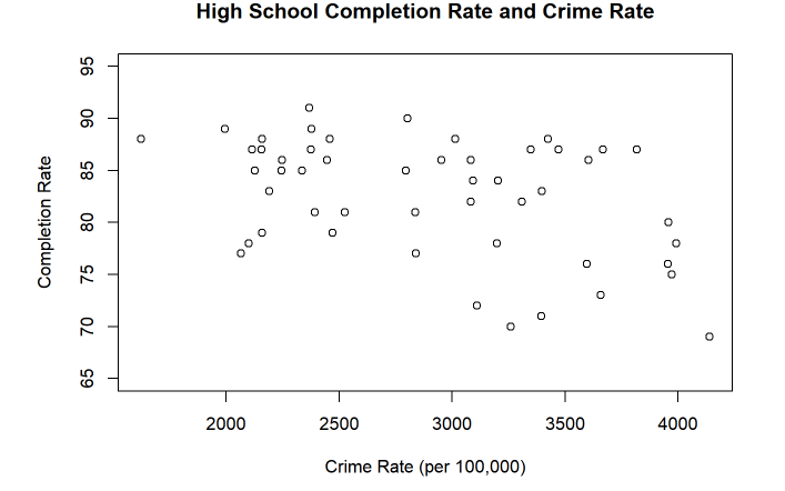
Read more about programming scatterplots here.
Hypothesis Testing
z-Test
-
Unless you choose to install a package in R, you will have to create your own z-test. There are a number of ways to accomplish this, but one way is to make a function that calculates the z-score and a separate command to calculate the P-value. In this case we are using the parameters for (x.bar), μ (mu), 𝜎 (sd), and number (n) for our z-test. To calculate the z-score, we use the equation:
.
> z.score = function(x.bar, mu, sd, n){
z <- ((x.bar-mu)/(sd/sqrt(n)))} greater than z score equals function left parenthesis x bar, mu, sd, n right parenthesis left curly bracket z less than minus left parenthesis left parenthesis x bar minus mu right parenthesis divided by left parenthesis sd divided by sqrt left parenthesis n right parenthesis right parenthesis right parenthesis right curly brackets -
Now plug in the values for the z-score function. Saving it as a new output will be useful for calculating the P-value and other test statistics.
> z_output <- z.score(16200,16000,2500,1000) greater than z underscore output less than minus z score left parenthesis Sixteen Thousand Two Hundred,Sixteen Thousand,Two thousand five hundred,One Thousand right parenthesis
>z_outputgreater than z underscore output
[1] 2.529822 -
Calculate the P-value for P( z ≥ 2.53) = P( z ≤ -2.53). As always, be careful to correctly evaluate the P-value depending on if you want the upper, lower, or two-tailed probability. Then evaluate if the p-value convinces you to reject or fail to reject the null hypothesis.
>p=pnorm(-z_output)greater than p equalspnorm left parenthesis minus z underscore output right parenthesis
>pgreater than p
## [1] 0.005706018 alpha = 0.01alpha equals zero point zero one
if (alpha > p) {if left parenthesis alpha greater than p right parenthesis left curly bracket
print("Reject null hypothesis")print left parenthesis Reject null hypothesis right parenthesis
} else { right curly bracket else left curly bracket
print ("Fail to reject the null hypothesis")print left parenthesis Fail to reject the null hypothesis right parenthesis
}right curly bracket
[1] "Reject null hypothesis"
Read more about z-tests here.
t-Test
-
There is a t.test option in R, but without a vector or list of data, it is necessary to create your own function. There are several ways to accomplish this, but one way is to make a function that calculates the t-score and a separate command to calculate the P-value. In this case we are using the parameters for (x.bar), μ0 (mu), s (s), and number (n) for our t-test. To calculate the t-score, we use the equation:
.
> t.score = function(x.bar, mu, s, n){
t <- ((x.bar-mu)/(s/sqrt(n)))} greater than t score equals function left parenthesis x bar, mu, s, n right parenthesis left curly bracket t less than minus left parenthesis left parenthesis x bar minus mu right parenthesis divided by left parenthesis s divided by sqrt left parenthesis n right parenthesis right parenthesis right parenthesis right curly bracket -
Now plug in the values for the t-score function. Saving it as a new output will be useful for calculating the p-value and other test statistics.
>t_output <- t.score(29,35,8,20)greater than t underscore output less than minus t score left parenthesis twenty nine, thirty five, eight, twenty right parenthesis
>t_outputgreater than t underscore output
[1] -3.354102 -
Calculate the P-value. As always, be careful to correctly evaluate the P-value depending on if you want the upper, lower, or two-tailed probability. Then evaluate if the P-value convinces you to reject or fail to reject the null hypothesis.
>alpha = 0.01greater than alpha equals zero point zero one
>p=2*pt(t_output, df=19)greater than p equals 2 asterisk times pt left parenthesis t underscore output, df equals nineteen right parenthesis
>pgreater than p
## [1] 0.003332838 if (alpha > p) {if left parenthesis alpha greater than p right parenthesis left curly braces
print("Reject null hypothesis")print left parenthesis Reject null hypothesis right parenthesis
} else { right curly bracket else left curly bracket
print ("Fail to reject the null hypothesis")print left parenthesis Fail to reject the null hypothesis right parenthesis
}right curly bracket
[1] "Reject null hypothesis"
Read more about t-tests here.
Normal Distribution
Normal Probability (cdf)
-
Use the function pnorm(z/x, mean = mu, sd = standard deviation, lower.tail = TRUE)pnorm left parenthesis z divided by x, mean equals mu, sd equals standard deviation, lower tail equasl True
Z/xZ divided by x : provide the z score or x value
mumu : if left off assumed to be 0
standard deviationstandard deviation: if left off assumed to be 1
lower.taillower tail: TRUETrue if left off. Include lower.tail = FALSElower tail equals False if you need the probability of observing a value above the x or z you provided.
Examples
-
> pnorm(1.37, lower.tail = FALSE)greater than pnorm left parenthesis one point three seven lower tail equals False right parenthesis
[1] 0.08534345 -
> pnorm(1.37)greater than pnorm left parenthesis one point three seven right parenthesis
[1] 0.9146565 -
with mean 25 and standard deviation 10
> pnorm(50,mean=25,sd=10)greater than pnorm left parenthesis fifty, mean equals twenty five, sd equals ten right parenthesis
[1] 0.9937903
Poisson Distribution
Poisson Probability (cdf)
-
Enter ppois(1, lambda=mean)ppois left parenthesis one, lambda equals mean right parenthesis. The probability is shown in output row [1].
> ppois(1,lambda=0.5)greater than ppois left parenthesis one, lambda equals zero point five right parenthesis
[1] 0.909796
Poisson Probability (pdf)
-
Enter dpois(x, lambda=mean)dpois left parenthesisx, lambda equals mean right parenthesis. The probability is shown in output row [1].
> dpois(0, lambda = .5)greater than dpois left parenthesis zero, lambda equals point five right parenthesis
[1] 0.6065307
Regression
Confidence Intervals for Slope and y-Intercept
To find the confidence interval for the slope and y-intercept of a linear regression, run your regression using the lm()lm left parenthesis right parenthesis function, then use the confint()confint left parenthesis right parenthesis function. Inside of this you give the model, and the confidence level desired.
> Y = c(12, 11, 12, 12, 13, 16, 13, 18, 11, 14)greater than Y equals c left parenthesis twelve, eleven, twelve, twelve, thirteen, sixteen, thirteen, eighteen, eleven, fourteen right parenthesis
> X = c(50, 51, 62, 45, 63, 76, 53, 68, 51, 74)greater than X equals c left parenthesis fifty, fifty one, sixty two, forty five, sixty three, seventy six, fifty three, sixty eight, fifty one, seventy foru right parenthesis
> model = lm(Y~X)greater than model equals lm left parenthesis Y tilde X right parenthesis
> confint(model,level=0.95)greater than confint left parenthesis model, level equals zero point nine five right parenthesis
| 2.5 % | 97.5 % | |
| (Intercept) | −2.74485180 | 10.9761507 |
| X | 0.03920706 | 0.2671791 |
Read more about confidence intervals here.
Correlation Coefficient
Revisiting the scatterplot we made previously (see Graphs > Scatterplot for information on the data set) , we can calculate its correlation using cor( x, y)cor left parenthesis x, y right parenthesis. The ouput indicates a moderately negative correlation which makes sense given the scatterplot.
> cor(School_and_crime$Crime.Rate..per.100.000,school_and_crime$High.School.Completion)greater than cor left parenthesis School underscore and underscore crime dollar Crime Rate dot dot per Hudred, school underscore and underscore crime dollar High School Completion right parenthesis
| [1] | -0.4262846 |
Regression Prediction Intervals
To find the confidence interval for the mean value of y given x, run your regression, then use the predict()predict left parenthesis right parenthesis function. Inside of this you give the model, the data to predict on as shown below, the type of interval, and the confidence level desired. For a simple linear regression, still use the newdata=list()newdata equals list left parenthesis right parenthesis notation.
> daughter <- c(65, 65, 61, 69, 67, 59, 69, 70, 68, 70, 70, 65, 70)greater than daughter less than minus c left parenthesis sixty five, sixty five, sixty one, sixty nine, sixty seven, fifty nine, sixty nine, seventy, sixty eight, seventy, seventy, sixty five, seventy right parenthesis
> mother <- c(64, 66, 62, 70, 70, 58, 66, 66, 64, 67, 65, 66, 68)greater than mother less than minus c left parenthesis sixty four, sixty six, sixty two, seventy, seventy, fifty eight, sixty six, sixty six, sixty four, sixty seven, sixty five, sixty six, sixty eight parenthesis
> father <- c(73, 70, 72, 72, 72, 63, 75, 75, 72, 69, 77, 70, 74)greater than father less than minus c left parenthesis seventy three, seventy, seventy two, seventy two, seventy two, sixty three, seventy five, seventy five, seventy two, sixty nine, seventy seven, seventy, seventy four right parenthesis
> m1 <- lm(daughter~mother+father)greater than m1 less than minus lm left parenthesis daughter tilde mother plus father right parenthesis
> predict(m1,newdata=list(mother=64, father=74),interval="confidence",level=0.95)greater than predict left parenthesis m1, newdata equals list left parenthesis mother equals seventy four, father equals seventy four right parenthesis, interval equals confidence, level equals zero point nine five right parenthesis
| fit | lwr | upr | |
| 1 | 66.82968 | 64.7847 | 68.87465 |
To find the predicted value of y given x, change the interval type to prediction.
> daughter <- c(65, 65, 61, 69, 67, 59, 69, 70, 68, 70, 70, 65, 70)greater than daughter less than semicolon minus c left parenthesis sixty five, sixty five, sixty one, sixty nine, sixty seven, fifty nine, sixty nine, seventy, sixty eight, seventy, seventy, sixty five, seventy right parenthesis
| fit | lwr | upr | |
| 1 | 66.82968 | 61.5329 | 72.12646 |
Read more about predictions here.
Simple Linear Regression
-
Create a list of values (vectors) for the x and y variables. Age will go on the x-axis and AskingPrice on the y-axis for this example.
> Age <- c(1,1,2,2,2,3,3,4,4,5,5,6,6,6)greater than Age less than minus c left parenthesis one, one, two, two, two, three, three, four, four, five, five, six, six, six right parenthesis
> AskingPrice <- c(17850,18000,15195,16995,15625,14935,14879,14460,13586,13050,13495,9150,9950,10995)greater than Asking Price less than minus c left parenthesis seventeen thousand eight hundred fifty, eighteen thousand, fifteen thousand one hundred ninety five,sixteen thousand nine hundred ninety five, fifteen thousand six hundred twenty five, fourteen thousand nine hundred thirty five, fourteen thousand eight hundred seventy nine,fourteen thousand four hundred sixty, thirteen thousand five hundred eighty six, thirteen thousand fifty, thirteen thousand four hundred ninety five, nine thousand one hundred fifty, nine thousand nine hundred fifty, ten thousand nine hundred ninetyfive right parenthesis -
Create a regression line using the command lm(y ~ x)lm left parenthesis y tilde x right parenthesis for linear model.
> RegressionLine <- lm(AskingPrice ~ Age)greater than Regression Line less than minus lm left parenthesis Asking Price tilde Age right parenthesis
-
Plot the points with the fitted linear model. The lines ()left parenthesis right parenthesis function can be used and the points should be sorted by the x-variable before being fit to the regression line.
> plot(Age, AskingPrice,xlab=greater than plot left parenthesis Age, AskingPrice, xlab equals"Age (Years)"Age left parenthesis Years right parenthesis,ylab=, ylab equals"AskingPrice"Asking Price,main=, main equals"Asking Price versus Age (Years)"Asking Price versus Age left parenthesis Years right parenthesis, lines(sort(Age),fitted(RegressionLine))), lines left parenthesis sort left parenthesis Age right parenthesis, fitted left parenthesis Regression Line right parenthesis right parenthesis right parenthesis
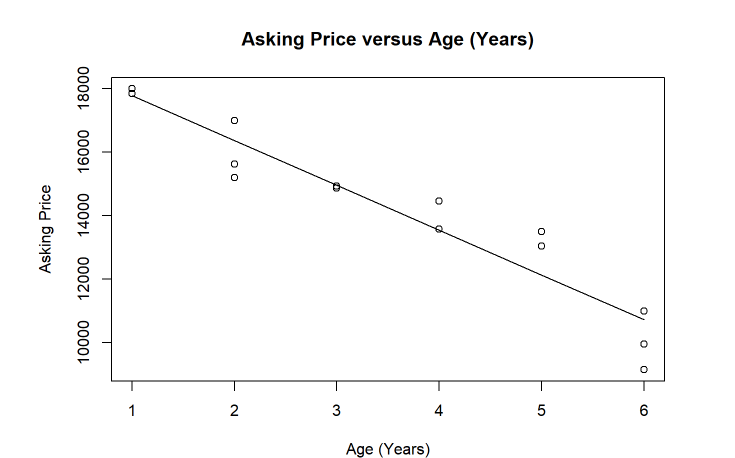
-
To get a summary of the linear regression line use summary ()left parenthesis right parenthesis function.
> summary(RegressionLine)greater than summary left parenthesis Regression Line right parenthesis
lm(formula = AskingPrice ~ Age)lm left parenthesis formula equals AskingPrice tilde Age right parenthesis
Residuals:Residuals colonMin 1Q Median 3Q Max -1574.94 -582.30 50.25 533.37 1357.83
Coefficients:Coefficients colonEstimate Std. Error t value Pr(>|t|) (Intercept) 19198.3 524.9 36.58 1.12e-13 Age -1412.2 131.8 -10.71 1.69e-07
---minus minus minus
Signif. codes: 0 '***' 0.001 '**' 0.01 '*' 0.05 '.' 0.1 ' ' 1Signif codes colon zero asterisk asterisk asterisk zero point zero zero one asterisk asterisk zero point zero one asterisk zero point zero five period zero point one single quotes open single quotes close one
Residual standard error: 868.7 on 12 degrees of freedomResidual standard error colon eight hundred sixty eight point seven on twelve degrees of freedom
Multiple R-squared: 0.9053, Adjusted R-squared: 0.8975Multiple R minus squared colon zero point nine zero five three, Adjusted R minus squared zero point eight nine seven five
F-statistic: 114.8 on 1 and 12 DF, p-value: 1.692e-07F minus statistic colon one hundred fourteen point eight on one and twelve DF, p minus value colon one point six nine two e minus zero seven
Read more about simple linear regression and plotting linear regression points here: Simple Linear Regression | The Default Scatterplot Function.
Sampling
Random Samples
See examples below. Enter the values you would like to sample from in an array named as you like. sample(x)sample left parenthesis x right parenthesis will sample from the given array without replacement and generate a sample with as many values as are in the array. By default, the function samples without replacement but you may specify replace=TRUEreplace equals True.
Example 1
> x<-c(1,2,3,5,6,7)greater than x less than minus c left parenthesis one, two, three, five, six, seven right parenthesis
> sample(x)greater than sample left parenthesis x right parenthesis
[1] 1 7 2 3 5 6
> sample(x, replace=TRUE)greater than sample left parenthesis x, repace equals True right parenthesis
[1] 3 5 5 3 2 1
> sample(x,2)greater than sample left parenthesis x, 2 right parenthesis
[1] 1 5
Example 2
> x <-1:5greater than x less than negative one colon five
> sample(x)greater than sample left parenthesis x right parenthesis
[1] 1 3 2 4 5
> sample(x,4,replace=TRUE)greater than sample left parenthesis x, 4, replace equals True right parenthesis
[1] 4 4 2 2
t-Distribution
Inverse t
-
Enter qt(probability, "df=" degrees of freedom)qt left parenthesis probability, df equals degrees of freedom right parenthesis. The t-value is shown in output row [1].
> qt(0.975, df=18)greater than qt left parenthesis zero point nine seven five, df equals 18 right parenthesis
[1] 2.100922
Hypergeometric Distribution
Hypergeometric Distribution
To find the probability of successes P(X=0)P left parenthesis x equals zero right parenthesis, P(X=1)P left parenthesis x equals 1 right parenthesis, and P(X=2)P left parenthesis x equals 2 right parenthesis, use the dhyper(number of successes in the sample of size n, number of possible successes, number of possible failures, number of draws) function. This can equivalently be written as dhyper(x, k, N-k, n)dhyper left parenthesis x, k, N minus k, n.
> dhyper(0,2,28,16)greater than dhyper left parenthesis zero,two,twenty eight,sixteen right parenthesis
## [1] 0.2091954
> dhyper(1,2,28,16)greater than dhyper left parenthesis one,two,twenty eight,sixteen right parenthesis
## [1] 0.5149425
> dhyper(2,2,28,16)greater than dhyper left parenthesis two,two,twenty eight,sixteen right parenthesis
## [1] 0.2758621
Read more about hypergeometric distributions here.