Minitab
ANOVA
One-Way
-
Enter the data for the different groups into separate columns.
-
Under StatStat, choose ANOVAANOVA, then One-wayOne minus way.
-
In the dropdown select Response data are in a separate column for each factor level.
-
Click the mouse in the box labeled Responses. Highlight the appropriate columns in the box on the left. Click Select.
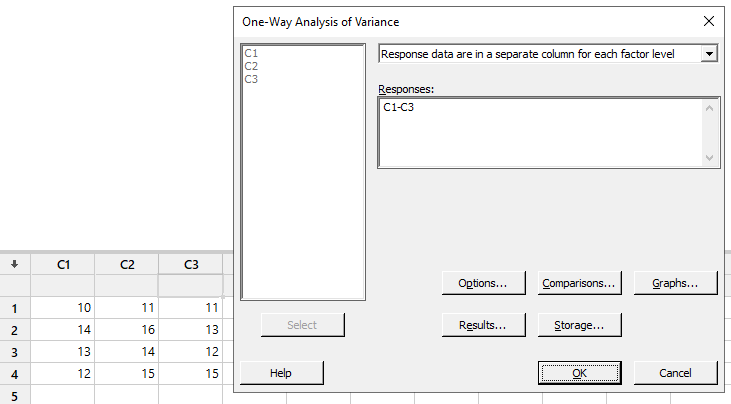
-
Press Options. Change Confidence level if desired.
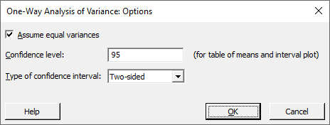
-
Press OK and OK.
One-way ANOVA: C1, C2, C3
Method
Null hypothesis All means are equal Alternative hypothesis Not all means are equal Significance level α = 0.05 Equal variances were assumed for the analysis. Factor Information
Factor Levels Values Factor 3 C1, C2, C3 Analysis of Variance
Source DF Adj SS Adj MS F-Value P-Value Factor 2 6.500 3.250 0.93 0.430 Error 9 31.500 3.500 Total 11 38.000 Model Summary
S R-sq R-sq(adj) R-sq(pred) 1.87083 17.11% 0.00% 0.00% Means
Factor N Mean StDev 95% CI C1 4 12.250 1.708 (10.134, 14.366) C2 4 14.00 2.16 (11.88, 16.12) C3 4 12.750 1.708 (10.634, 14.866) Pooled StDev = 1.87083
Fisher's LSD
-
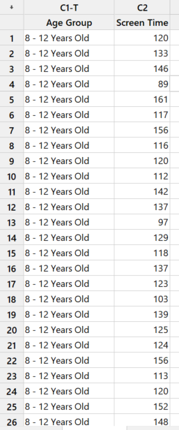
Enter the category labels in Column C1. Enter the corresponding data value in Column C2.
-
Choose Stat, ANOVA, and One-Way.
-
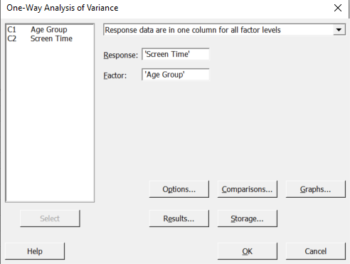
Enter the data for the Response and the categories for the Factor. Select OptionsOptions and enter the desired Confidence levelConfidence level. Press OKOK.
-
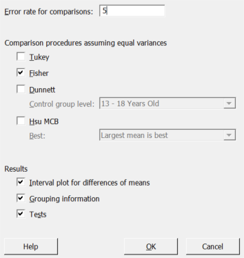
Click on ComparisonsComparisons and check the box for FisherFisher and for TestsTests. Press OKOK. Press OKOK again.
-
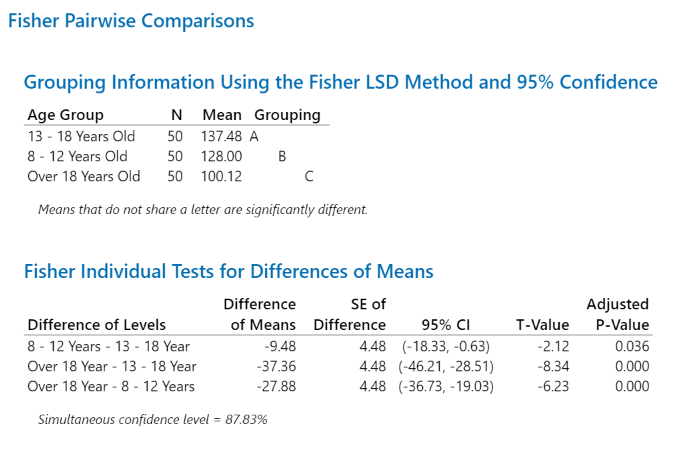
Observe the results of Fisher's LSD test.
Tukey's HSD
-
Enter the category labels in Column C1. Enter the corresponding data value in Column C2.
-
Choose StatStat, ANOVAANOVA, and One-wayOne minus way.
-
Enter the data for the Response and the categories for the Factor. Select OptionsOptions and enter the desiredConfidence levelConfidence level. Press OKOK.
-
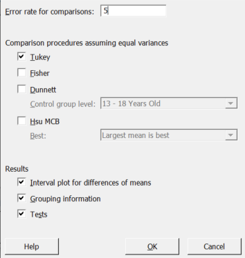
Click on Comparisons and check the box for TukeyTukey and for TestsTests. Press OKOK. Press OKOK again.
-
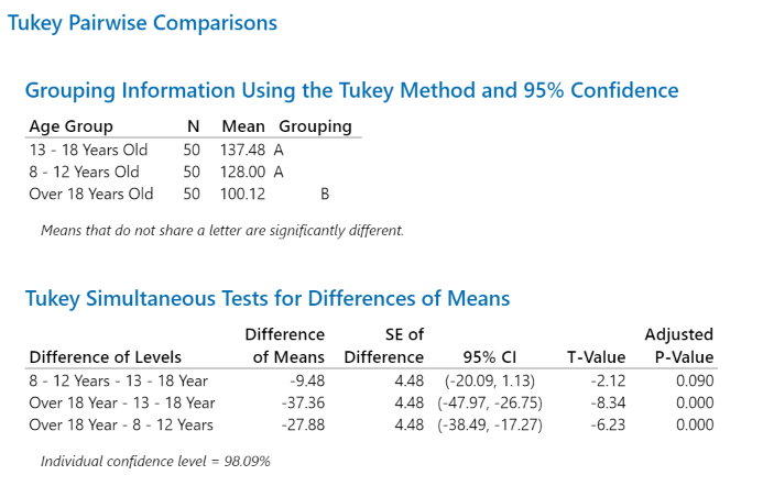
Observe the results of Tukey's HSD test.
Two-Way
-
Enter all the data into C1, one column at a time. Enter the row numbers into C2 and the column numbers into C3. Label the columns as is fitting.
-
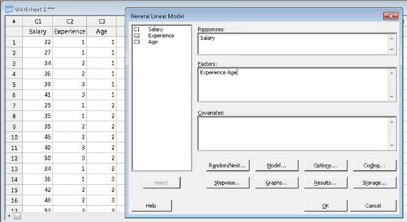
Under StatStat, choose ANOVAANOVA, then General Linear ModelGeneral Linear Model, then Fit General Linear Model…Fit General Linear Model horizontal ellipsis.
-
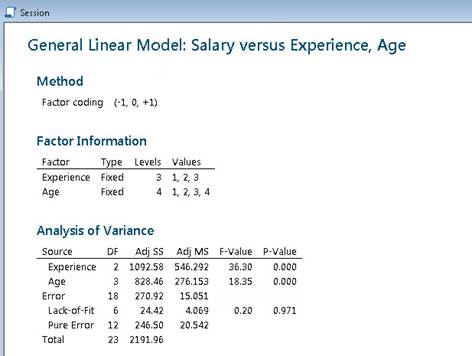
Use select to input C1 as Responses and C2, C3 as Factors. Select OKOK.
Binomial Distribution
Binomial Probability Distribution
-
Set up the worksheet in C1 and C2 as shown below.
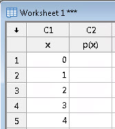
-
Press CalcCalc,Probability DistributionsProbability Distributions, and BinomialBinomial.
-
Designate Probability. (Alternatively, Cumulative Probability)
-
Complete the dialog box with Number of trials – "12", Event probability – "0.1", Input column – "x", and Optional storage – "p(x)".
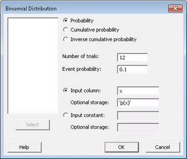
-
Press OKOK and read output in C2.
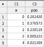
Chi-Square Distribution
Critical Value
-
Enter the area to the left of the desired critical value in the first row of column C1C1. If the area we are given is to the right of the critical value, we must first determine the area to the left by calculating (1-area to the right).
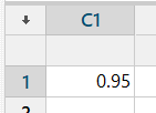
-
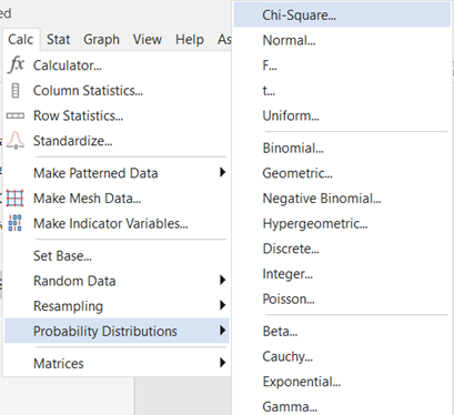
Go to CalcCalc,Probability DistributionsProbability Distributions, Chi-SquareChi Square.
-
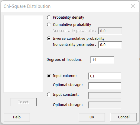
Choose Inverse cumulative probabilityInverse cumulative probability and enter the number for Degrees of freedomDegrees of freedom. Select C1C1 as the input column.
-
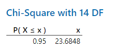
Click OKOK and the critical value will appear in the Session window.
Left Tailed Probability (cdf)
-
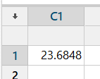
Enter the Chi-Square value in the first row of column C1C1.
-
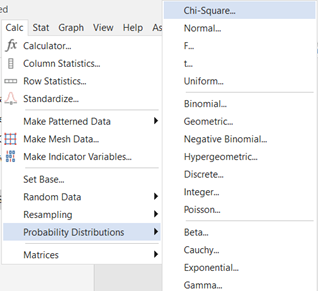
Go to CalcCalc,Probability DistributionsProbability Distributions, Chi-SquareChi minus Square.
-
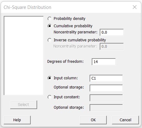
Select Cumulative ProbabilityCumulative Probability and enter the number for Degrees of freedomDegrees of freedom. Select C1C1 as the input column.
-
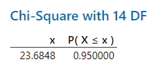
Click OKOK and the probability will appear in the Session window.
Test for Association
-
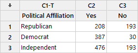
Input the data in the Worksheet.
-
Choose StatStat, TablesTables, and Chi-Square Test for AssociationChi minus Square Test for Association.
-
Select Summarized data in a two-way tableSummarized data in a two way table from the dropdown.
-
Under Columns containing the table, input column "C2 Yes" and column "C3 No". Press OK.
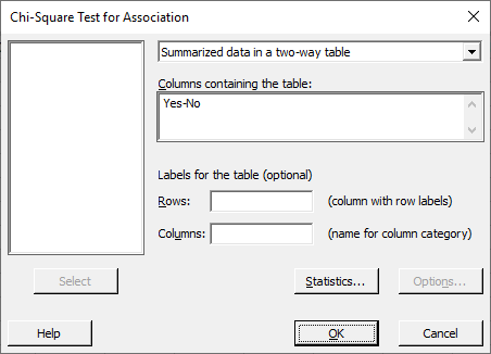
Chi-Square Test for Association: Worksheet rows, Worksheet columns
Rows: Worksheet rows Columns: Worksheet columns
Yes No All 1 208
288.8193
112.2417 2 387
300.330
116.7417 3 476
481.8193
187.2669 All 1071 416 1487 Cell Counts
Count
Expected countChi-Square Test
Chi-Square DF P-Value Pearson 170.467 2 0.000 Likelihood Ratio 187.856 2 0.000 Note: The first row (labeled ‘Pearson’) under Chi-Square Test in the output corresponds to the methods used in the texts.
Test for Goodness of Fit
-
Input the data in the Worksheet.
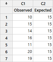
-
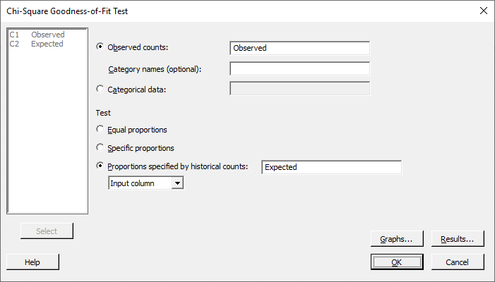
Choose StatStat, TablesTables, and Chi-Square Goodness-of-Fit Test (One Variable)...Chi Square Goodness of Fit Test left parenthesis One Variable right parenthesis...
-
Select your Observed column for Observed countsObserved counts.
-
Select Proportions specified by historical countsProportions specified by historical counts and choose your Expected column as the Input column. Press OKOK.
Chi-Square Goodness-of-Fit Test for Observed Counts in Variable: Observed
Observed and Expected Counts
Category Observed Historical
CountsTest
ProportionExpected Contribution
to Chi-Square1 10 15 0.142857 15 1.66667 2 15 15 0.142857 15 0.00000 3 14 15 0.142857 15 0.06667 4 16 15 0.142857 15 0.06667 5 11 15 0.142857 15 1.06667 6 20 15 0.142857 15 1.66667 7 19 15 0.142857 15 1.06667 Chi-Square Test
N DF Chi-Sq P-Value 105 6 5.6 0.469
Confidence Intervals
Proportion
-
Choose StatStat, select Basic StatisticsBasic Statistics and then choose 1 ProportionOne Proportion.
-
Select Summarized dataSummarized data from the dropdown and enter Number of events and Number of trials.
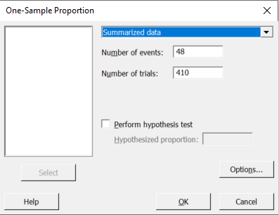
-
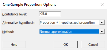
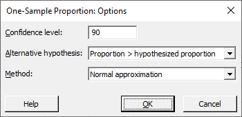
Click the OptionsOptions button. Enter the Confidence level and select Normal approximation from the second dropdown.
-
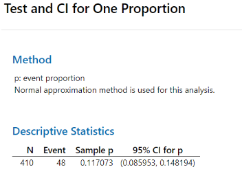
Press OKOK and press OKOK again.
t-Interval
-
Select StatStat, then Basic StatisticsBasic Statistics, and 1-Sample tOne Sample t.
-
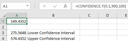
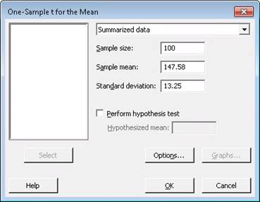
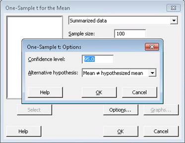
In the dropdown menu select Summarized dataSummarized data and input the sample size, mean, and standard deviation. (Or if you have the raw data, enter the data into into C1 and select One or more samples, each in a columnOne or more samples, each in a column from the dropdown menu and then select C1.)
-
Select OptionsOptions and choose your confidence level. For a confidence interval select a Mean ≠ hypothesized meanMean not equal to hypothesized mean as the alternative hypothesis from the dropdown menu.
-
Click OKOK on the Options window and OKOK on the main dialog window and the confidence interval is displayed in the Session window.
Two Sample t-Interval (Independent Samples)
-
Select StatStat, then Basic StatisticsBasic Statistics, and 2-Sample tTwo Sample less than em greater than t less than divided by em greater than.
-
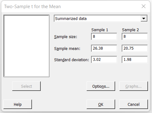
In the dropdown menu select Summarized dataSummarized data and input the sample size, sample mean, and sample standard deviation. (If you have the raw data, enter the data for the first sample into C1C1 and for the second sample into C2C2 and select Each sample is in its own column. Then select C1C1 for Sample 1Sample One and C2C2 for Sample 2Sample Two.)
-
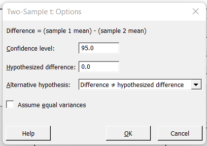
Select OptionsOptions and choose your Confidence levelConfidence level. For a confidence interval select Difference ≠ Hypothesized differenceDifference not equal to Hypothesized difference as the alternative hypothesis from the dropdown menu. If you assume the sample variances are equal, check the box Assume equal variancesAssume equal variances. Press OKOK. (Note the box was not checked for the results that follow.)
-
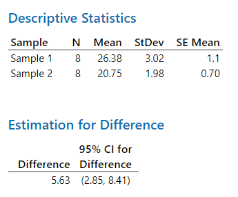
Press OKOK. The confidence interval is produced in the Session window.
Two Sample Proportions z-Interval
-
Go to Stat > Basic Statistics > 2 ProportionsStat greater than Basic Statistics greater than Two Proportions.
-
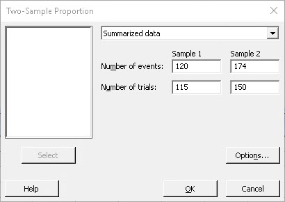
Choose Summarized data and enter x1 for Number of events for the Sample 1, and n1 for Number of trials. Then enter x2 for Number of events for the Sample 2 and n2 for Number of trials.
-
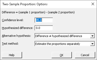
Choose OptionsOptions and enter the desired Confidence level.
-
Click OKOK on the Options and main dialog window and the confidence interval is displayed in the Session window.
Minimum Sample Size
-
Under the StatStat menu, select Power and Sample SizePower and Sample Size, and then select Sample Size for EstimationSample Size for Estimation
-
Select the ParameterParameter and then enter an estimate of the specified parameter for Planning Value.
-
You can use information from a previous study, subject-matter knowledge, design specifications, etc. to determine this Planning Value
-
-
In the second dropdown, choose Estimate sample sizesEstimate sample sizes and provide your desired Margins of error for confidence itervals.
-
Click Options…Options… and input the appropriate confidence level.
-
Click OKOK and OKOK.
Standard Deviation
-
Under the StatStat menu, select Basic StatisticsBasic Statistics, and then select 1 Variance...one Variance horizontal ellipse
-
Select Sample Standard DeviationSample Standard Deviation in the dropdown menu. Then, fill in the boxes labeled Sample size and Sample standard deviation.
-
Click on the button labeled Options...Options horizontal ellipse In the pop-up window that appears, specify the confidence level and Standard deviation ≠ hypothesized standard deviationStandard deviation not equal to hypothesized standard deviation for the Alternative hypothesisAlternative hypothesis.
-
Click OKOK on the Options window andOKOK on the main dialog window and the confidence interval is displayed in the Session window.
Variance
-
Under the StatStat menu, select Basic StatisticsBasic Statistics, and then select 1 Variance...One Variance horizontal ellipse
-
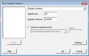
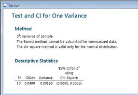
Select Sample VarianceSample Variance in the dropdown menu. Then, fill in the boxes labeled Sample size and Sample variance.
-
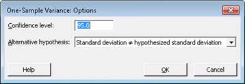
Click on the button labeled Options...Options horizontal ellipsis In the pop-up window that appears, specify the confidence level and Standard deviation ≠ hypothesized standard deviationStandard deviation not equal to hypothesized standard deviation for the ≠ Alternative hypothesis.
-
Click OKOK on the Options window and OKOK on the main dialog window and the confidence interval is displayed in the Session window.
z-Interval
-
Select StatStat, then Basic StatisticsBasic Statistics, and 1-Sample ZOne Sample Z.
-
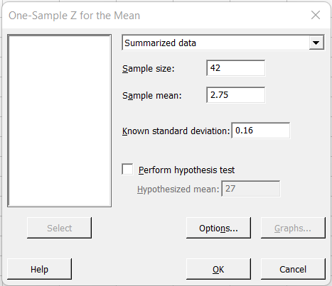
In the dropdown menu select Summarized dataSummarized data and input the sample size, sample mean, and known standard deviation. (If you have the raw data enter the data into C1C1 and select One or more samples, each in a columnOne or more samples, each in a column from the dropdown menu and then select C1C1.)
-
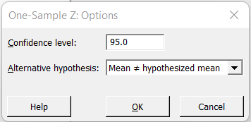
Click OptionsOptions and enter the desired Confidence levelConfidence level. For a confidence interval select a Mean ≠ alternative meanMean not equal to alternative mean as the Alternative hypothesisAlternative hypothesis from the dropdown menu. Press OKOK.
-
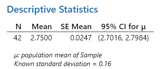
Press OKOK.
Counting
Combination
-
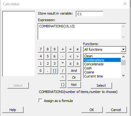
Go to Calc > Calculator.
-
Type C1 in the box after "Store result in variable:".
-
Select Combinations under the All functions drop down box and click Select.
-
Then input a number to replace "number of items" and a number to replace "number to choose" in the expression. For example, input 15 to replace "number of items" and 13 to replace "number to choose" in order to calculate 15C13.
-
Click OK. The result will be displayed in row 1 of column C1.
Factorial
-
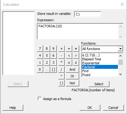
Go to Calc > Calculator.
-
Type C1 in the box after "Store result in variable:".
-
Select Factorial under the All functions drop down box and click Select.
-
Then input a number to replace "number of items" in the expression. For example, input 10 to calculate 10!
-
Click OK. The result will be displayed in row 1 of column C1.
Permutation
-
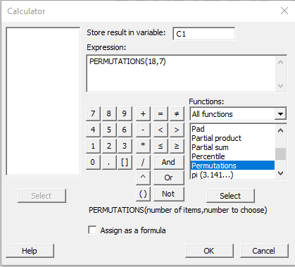
Go to Calc > Calculator.
-
Type C1 in the box after "Store result in variable:".
-
Select Permutations under the All functions drop down box and click Select.
-
Then input a number to replace "number of items" and a number to replace "number to choose" in the expression. For example, input 18 to replace "number of items" and 7 to replace "number to choose" in order to calculate 18P7.
-
Click OK. The result will be displayed in row 1 of column C1.
Descriptive Statistics
One Variable
-
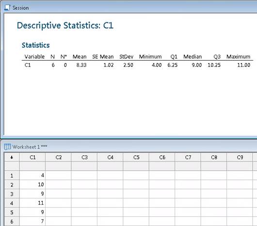
Enter the data into column C1.
-
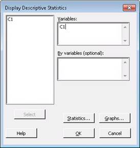
Under StatStat, choose Basic StatisticsBasic Statistics, then Display Descriptive StatisticsDisplay Descriptive Statistics.
-
In the dialog box, input "C1C1" under Variables.
-
Click StatisticsStatistics to select which statistics to include. Select OKOK.
-
Observe the Output Screen for the summary statistics.
F-Distribution
F Critical Value
-
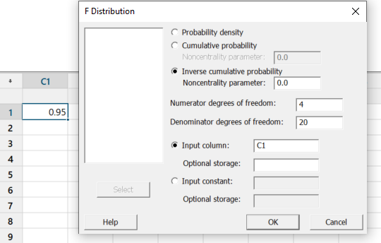
Enter the area to the left of the F critical value into cell C1,1C1, One.
-
Choose CalcCalc,Probability DistributionsProbability Distributions, and Inverse Distribution FunctionInverse Distribution Function.
-
Change DistributionDistribution to FF. Change Form of inputForm of input to 'A column of values'. Enter C1C1 for Values inValues in. Enter the desired numerator and denominator degrees of freedom. For OutputOutput select the radio button next to 'Display a table of inverse cumulative probabilities.' Press OKOK.
-
Observe the results.

F-Probability (cdf)
-
Enter the F critical value into cell C1,1C1, One.
-
Choose CalcCalc,Probability DistributionsProbability Distributions, and FF.
-
Select the radio button next to Cumulative ProbabilityCumulative Probability. Enter the desired numerator and denominator degrees of freedom. Select the radio button next to Input columnInput column and enter C1C1. Press OKOK.
-
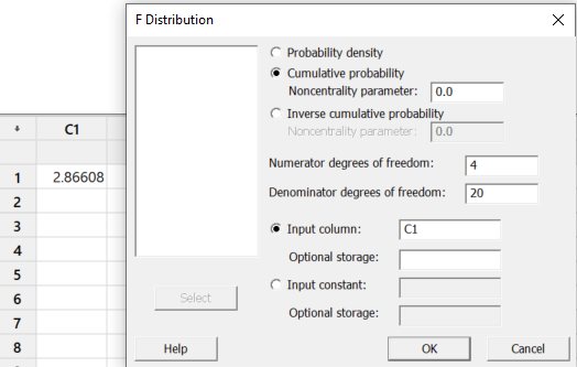
Note: You can also select Input constantInput constant and enter the F critical value there.

-
Observe the results.
Graphs
Bar Charts
-
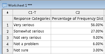
Enter the category labels in C1C1 and the corresponding data counts in C2C2. The axis labels can be entered in the column header.
-
Select Graph, Bar ChartGraph, Bar Chart.
-
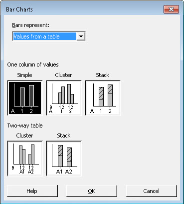
From the Bars represent:Bars represent colon dropdown, select Values from a tableValues from a table and ensure SimpleSimple is selected for One column of valuesOne column of values. Press OKOK.
-
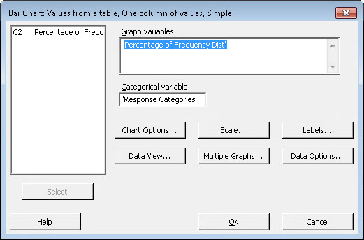
Select C2C2 for Graph variablesGraph variables and C1C1 for Categorical variableCategorical variable.
-
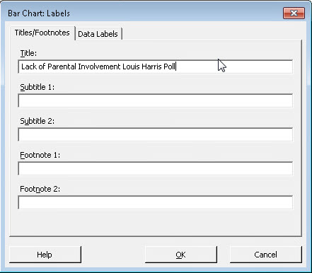
To add a title, select LabelsLabels and enter the title under TitleTitle.
-
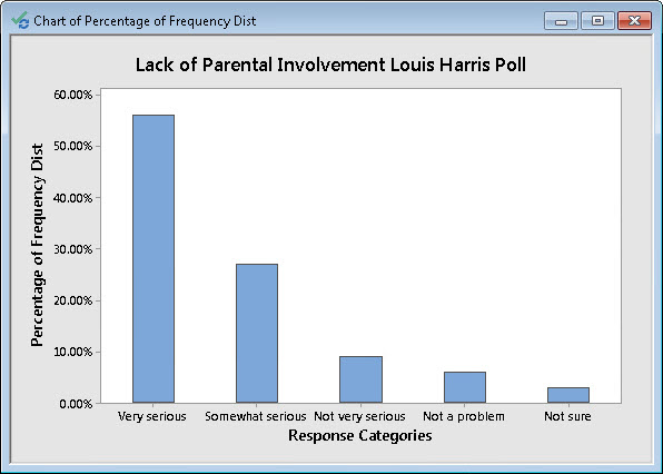
Press OKOK and OKOK.
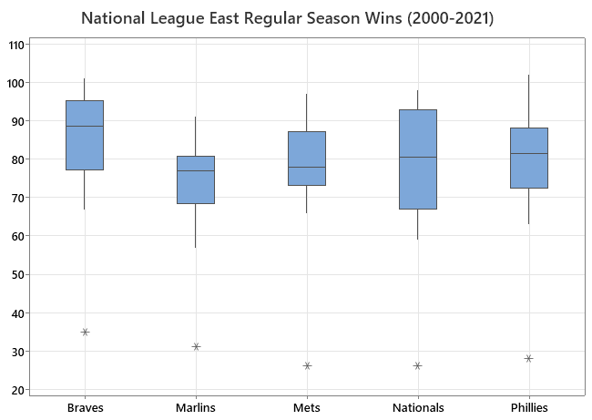
Boxplot
-
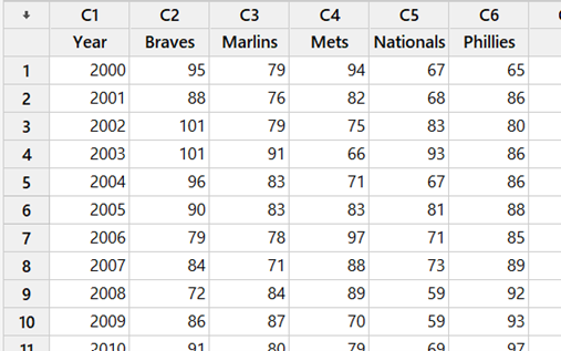
Enter the data for each box plot in a separate column. The column header can be used to display the label for each box plot.
-
Select Graph, BoxplotGraph, Boxplot.
-
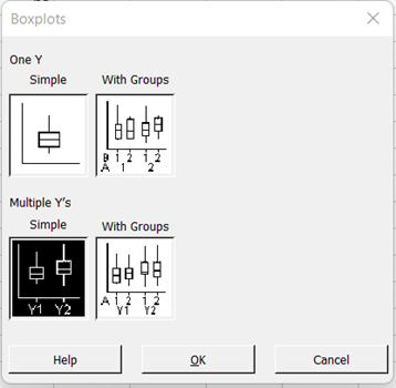
Select One Y, SimpleOne Y, Simple for a single data column or select Multiple Y's, SimpleMultiple Y apostrophe's, Simple for side-by-side boxplots for several data columns. Press OKOK.
-
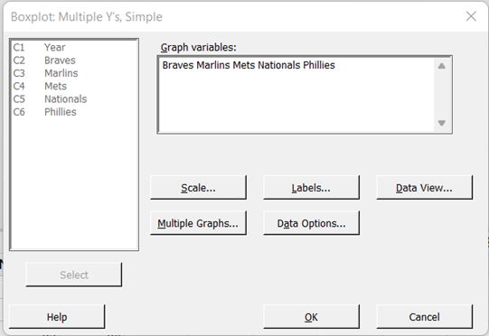
Select the appropriate column(s) for Graph variablesGraph variables.
-
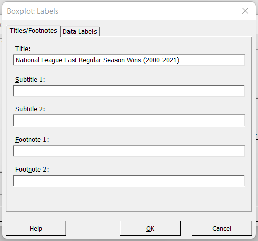
To add a title to the box plot, click LabelsLabels and enter the title under TitleTitle.
-
Click OKOK and OKOK.
Dot Plot
-
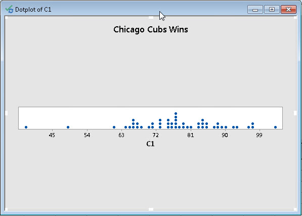
Enter the data into column C1.
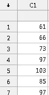
-
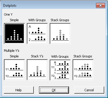
Select Graph, DotplotGraph, Dotplot.
-
Select One Y, SimpleOne Y, Simple and click OKOK.
-
Select C1 for Graph variablesGraph variables.
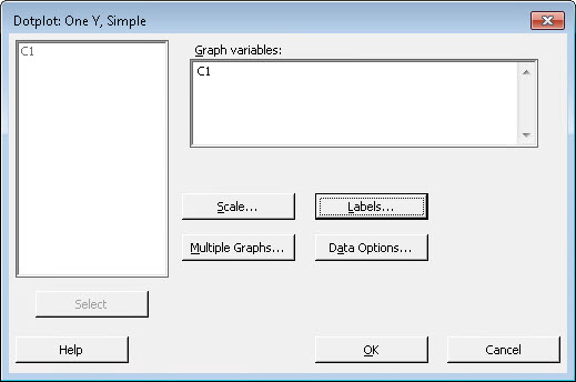
-
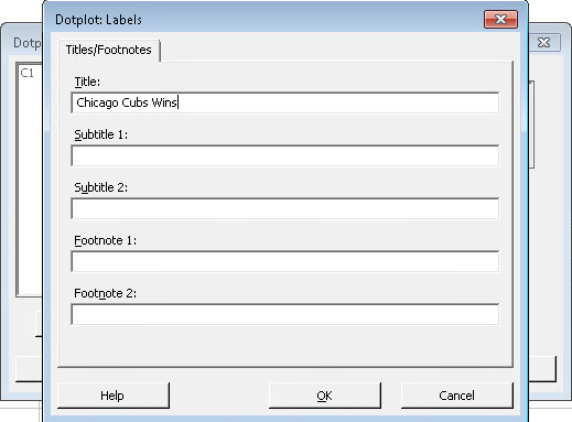
To add a title, click LabelsLabels and enter the title under TitleTitle.
-
Click OKOK and OKOK.
Histogram
-
Enter the data in the column, C1.
-
Select GRAPHGRAPH, HistogramHistogram.
-
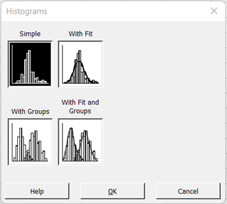
Select SimpleSimple. Press OKOK.
-
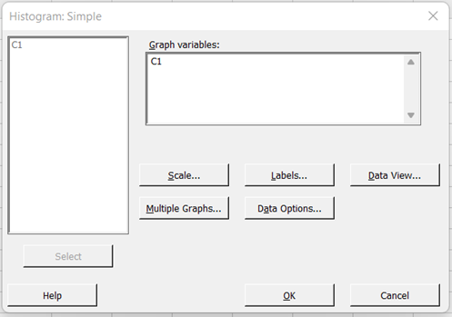
Select C1C1 for Graph variablesGraph variables.
-
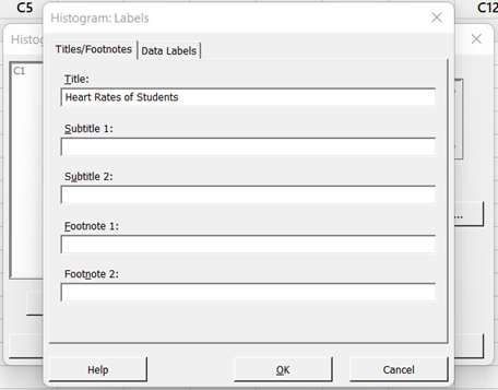
To add a title, choose LabelsLabels and enter the title under TitleTitle.
-
Press OKOK and OKOK to generate the graph.
-
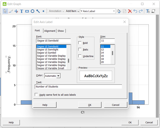
To edit the axis labels, double-click on the text along the axis. Double-click on the text again in the Edit GraphEdit Graph pop-up window. Type the text of the axis label in the Text:Text colon window.
-
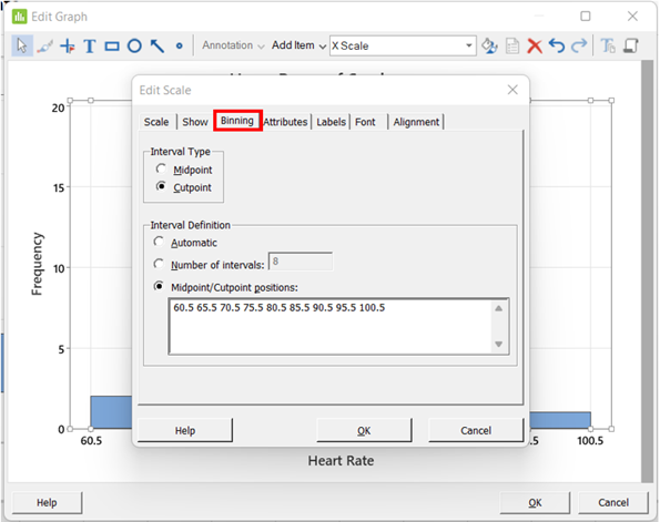
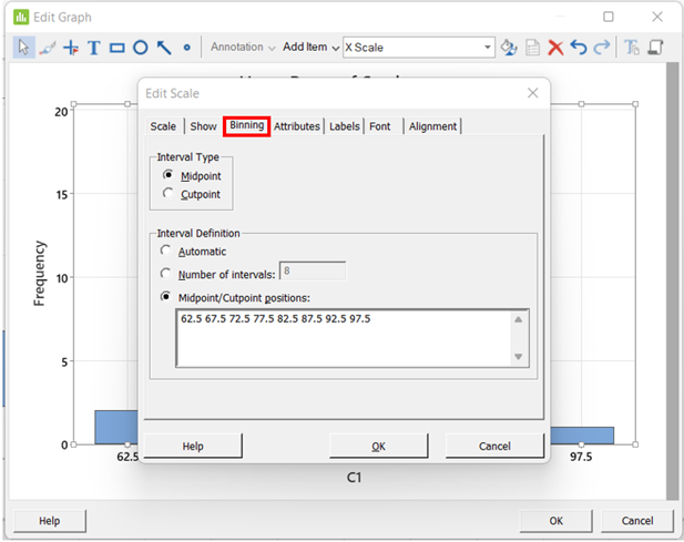
There are two options for how the classes are displayed along the horizontal axis. For either, double-click on one of the numbers on the x-horizontal axis. Double click on a horizontal axis number in the Edit Graph pop-up window. Select the Binning tab on the Edit Scale menu.
Option 1: Choose MidpointMidpoint for the Interval Type, select Midpoint/Cutpoint positionsMidpoint divided by Cutpoint positions under Interval Definition. Enter the midpoints of each class
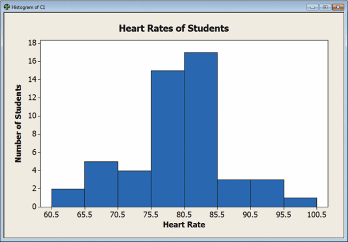
Option 2: Choose CutpointCutpoint for the Interval Type, select Midpoint/Cutpoint positionsMidpoint divided by Cutpoint positions under Interval Definition. Enter the upper class boundaries of each class
Line Graph
-
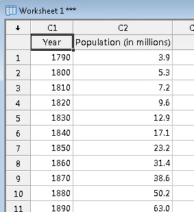
Enter the category labels in C1 and the corresponding data in C2. The axis labels can be entered in the header column. (Category labels are not required.)
-
Select Graph, Time Series PlotGraph, Time Series Plot .
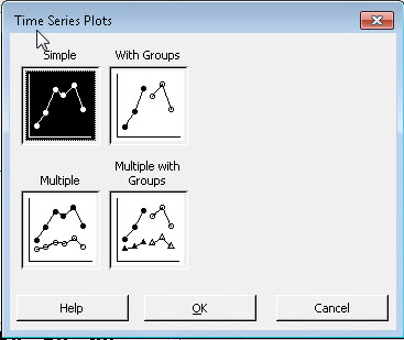
-
Select SimpleSimple and click OKOK.
-
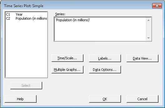
Select C2 for SeriesSeries.
-
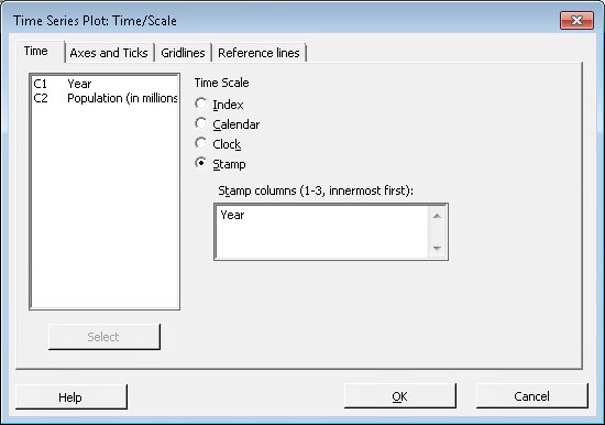
Select Time/ScaleTime divided by Scale and select StampStamp for Time ScaleTime Scale. Select C1 for Stamp columnsStamp columns. Press OKOK.
-
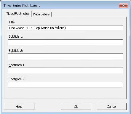
To add a title, click LabelsLabels and enter the title under TitleTitle.
-
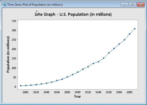
Click OKOK and OKOK.
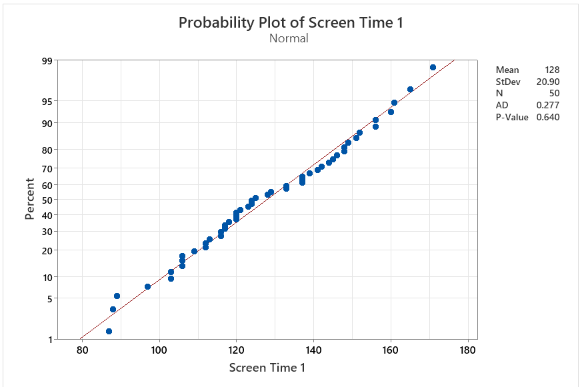
Normal Probability Plot
-
Input your data in C1.
-
Select GRAPHGRAPH, Probability PlotProbability Plot.
-
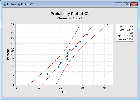
With Single selected press OKOK.
-
Input "C1C1" into Graph variables.
-
Press OKOK.
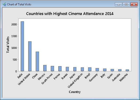
Pareto Chart
-
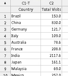
Enter the category labels in C1C1 and the corresponding data counts in C2C2. The axis labels can be entered in the column header.
-
Select Graph, Bar ChartGraph, Bar Chart.
-
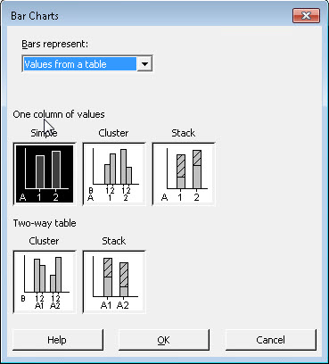
From the Bars represent:Bars represent colon dropdown, select Values from a tableValues from a table and ensure SimpleSimple is selected for One column of valuesOne column of values. Press OKOK.
-
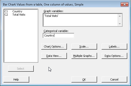
Select C2C2 for Graph variablesGraph variables and C1C1 for Categorical variableCategorical variable.
-
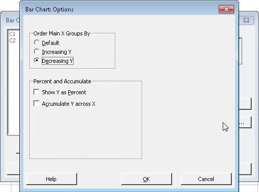
Select Chart OptionsChart Options and select Decreasing YDecreasing Y under Order Main X Groups ByOrder Main X Groups By.
-
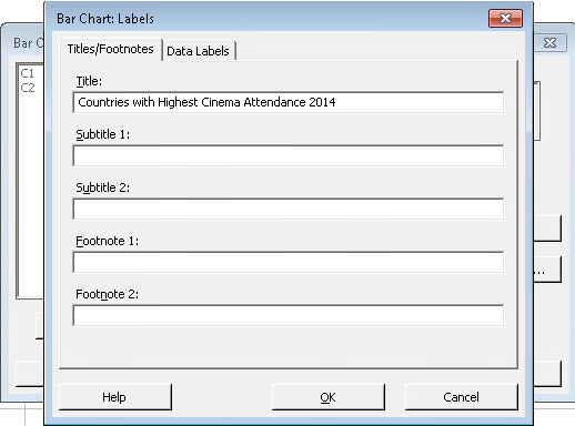
To add a title, select LabelsLabels and enter the title under TitleTitle.
-
Press OKOK and OKOK.
Pie Chart
-
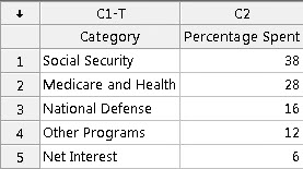
Enter the category labels in C1C1 and the corresponding data counts in C2C2.
-
Select Graph, Pie ChartGraph, Pie Chart
-
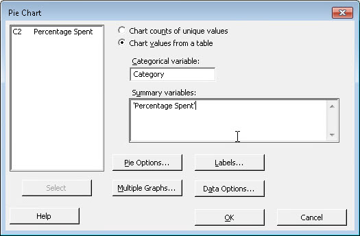
Select Chart values from a tableChart values from a table and select C1C1 for C1C1 and C2C2 for Summary variablesSummary variables.
-
To add a title, click LabelsLabels and enter the title under TitleTitle.
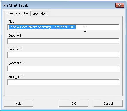
-
To display the percentages each slice represents on the graph, click Slice LabelsSlice Labels and choose PercentPercent.
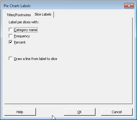
-
Click OKOK and OKOK.
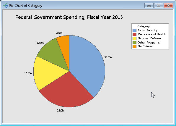
Scatterplot
-
Enter the data with the independent(explanatory) variable in C1C1 and the corresponding dependent(response) variable in C2C2. Add column headers if desired.
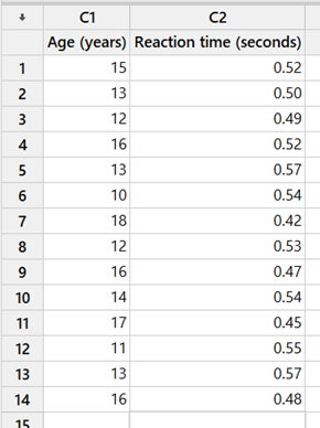
-
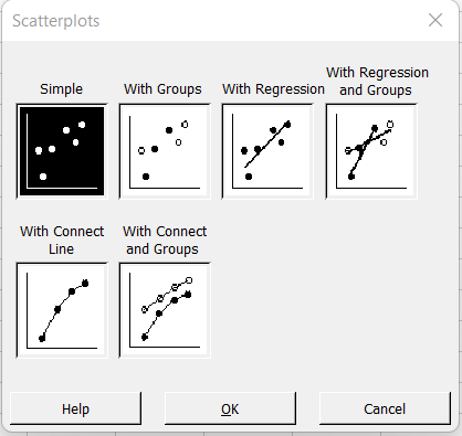
Select GRAPHGRAPH, ScatterplotScatterplot.
-
Select SimpleSimple. Press OKOK.
-
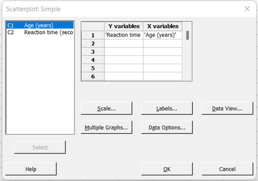
Select C2C2 for Y variablesY variables and C1C1 for X variablesx variables.
-
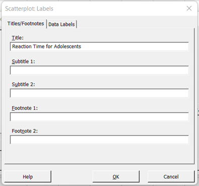
To add a title to the scatterplot, click LabelsLabels and enter the title under TitleTitle.
-
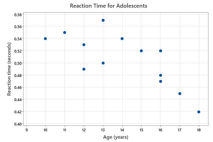
Press OKOK and OKOK.
Stem-and-Leaf Plot
-
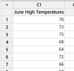
Enter the data in C1C1.
-
Select Graph, Stem-and-LeafGraph, Stem and Leaf
-
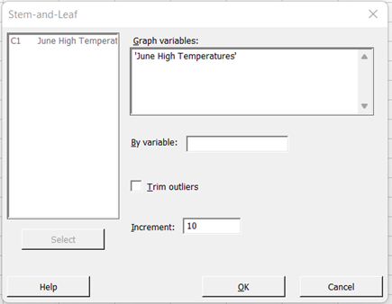
Select C1C1 for Graph variablesGraph variables and enter Increment:Increment colon value of the stems.
-
Press OKOK and OKOK.
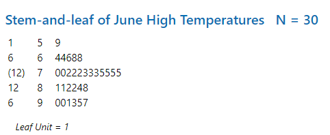
Note: The middle column is the stem with the rightmost column displaying the leaves. The first (leftmost) column contains cumulative counts. The count for the row that contains the median value is enclosed in parentheses. The count for a row above the median shows the total count for that row and all the rows above it. The value for a row below the median shows the total count for that row and all the rows below it.
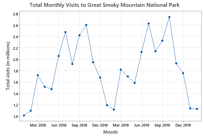
Time Series Plot
-
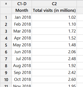
Enter the data with time periods in C1C1 and corresponding data in C2C2.
-
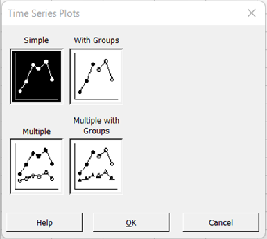
Select GRAPHGRAPH, Time Series PlotTime Series Plot.
-
Select SimpleSimple. Press OKOK.
-
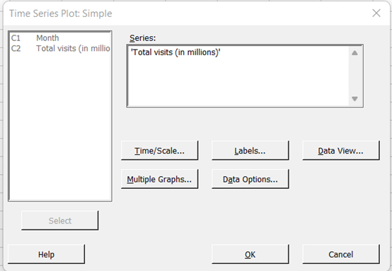
Select C2C2 for SeriesSeries.
-
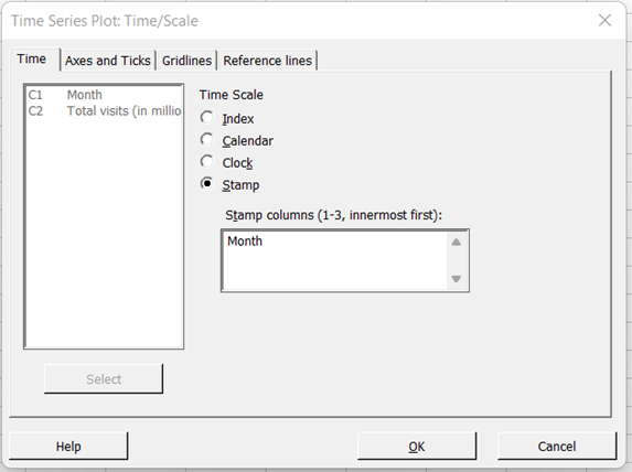
Click Time/ScaleTime divided by Scale and then choose StampStamp. Select C1C1 for Stamp columnsStamp columns. Press OKOK.
-
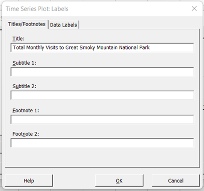
To add a title, choose click LabelsLabels and enter the title under TitleTitle.
-
Press OKOK and OKOK.
Hypothesis Testing
z-Test
-
Enter the sample data into column C1.
-
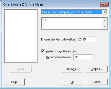
Choose Stat, Basic Statistics,Stat, Basic Statistics, and 1-Sample ZOne Sample Z. Select OptionsOptions to set the appropriate Alternative hypothesis and press OKOK.
-
Enter "C1C1" for Variables, and enter the Known standard deviation, if applicable. Check the box for Perform hypothesis testPerform hypothesis test and enter the Hypothesized mean. Press OKOK.
-
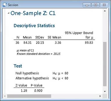
Observe the session window for the results.
One Proportion z-Test
-
Select StatStat, Basic StatisticsBasic Statistics, 1 ProportionOne Proportion.
-
From the dropdown choose Summarized dataSummarized data.
-
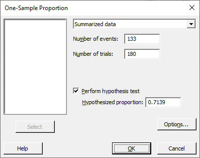
Enter the Number of eventsNumber of events and the Number of trialsNumber of trials. Check Perform hypothesis testPerform hypothesis test and enter a Hypothesized proportionHypothesized proportion.
-
Click OptionsOptions. Enter a Confidence level, select an Alternative hypothesisAlternative hypothesis, and choose Normal approximationNormal approximation for the MethodMethod.
-
Press OKOK and OKOK.
Test and CI for One Proportions
Method
p: event proportion Normal approximation method is used for this analysis. Descriptive Statistics
N Event Sample p 90% Lower Bound
for p180 133 0.738889 0.696932 Test
Null hypothesis H0: p = 0.7139 Alternative hypothesis H1: p > 0.7139 Z-Value P-Value 0.74 0.229
t-Test
Using Data
-
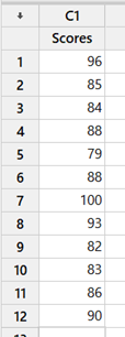
Enter the sample data into column C1C1.
-
Choose StatStat, Basic StatisticsBasic Statistics, and 1-Sample tOne Sample t.
-
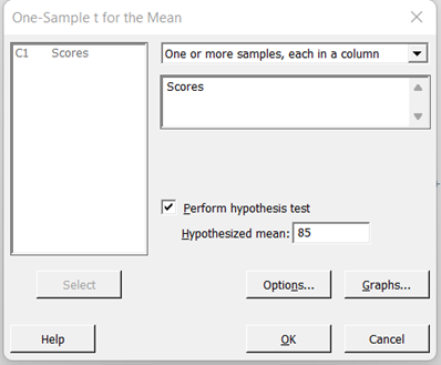
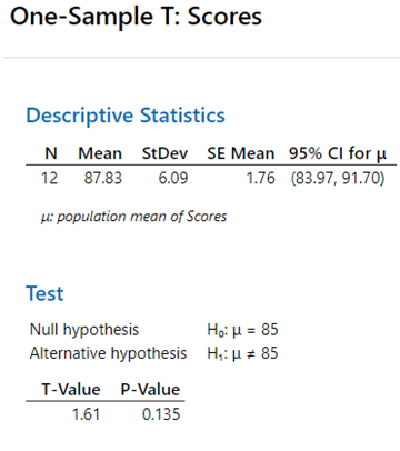
From the dropdown menu choose One or more samples, each in a columnOne or more samples, each in a column. Click in the empty window below the dropdown. Select "C1" for the variable. Check the box for Perform hypothesis testPerform hypothesis test and enter the value of the Hypothesized meanHypothesized mean.
-
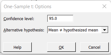
Select OptionsOptions to set the appropriate Confidence levelConfidence level and Alternative hypothesisAlternative hypothesis. Press OKOK.
-
Press OKOK.
Using Summary Statistics
-
Choose StatStat, Basic StatisticsBasic Statistics, and 1-Sample tOne Sample t.
-
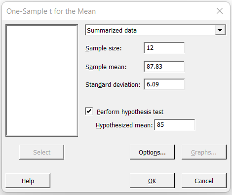
From the dropdown choose Summarized dataSummarized data. Enter the Sample sizeSample size, Sample meanSample mean, and the Standard deviationStandard deviation. Check Perform hypothesis testPerform hypothesis test and enter a value for the Hypothesized meanHypothesized mean.
-
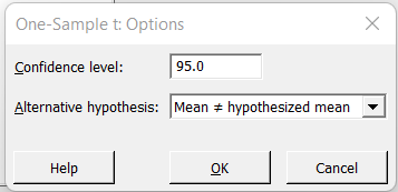
Select OptionsOptions to set the appropriate Confidence levelConfidence level and Alternative hypothesis.Alternative hypothesis. Press OKOK.
-
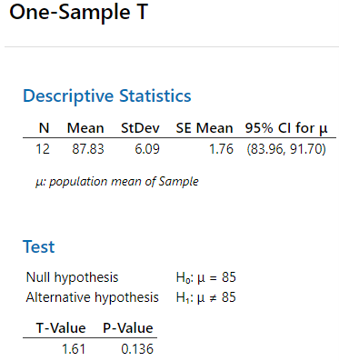
Press OKOK.
Two Proportion z-Test
Method: Summary Statistics
-
Select StatStat, Basic StatisticsBasic Statistics, 2 ProportionsTwo Proportions
-
From the dropdown choose Summarized dataSummarized data.
-
Enter the Number of eventsNumber of events and the Number of trialsNumber of trials for each sample.
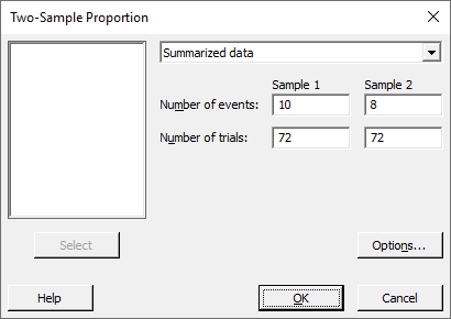
-
Choose OptionsOptions to adjust the Confidence levelConfidence level, Hypothesized differenceHypothesized difference, Alternative hypothesisAlternative hypothesis, and Test MethodTest Method.
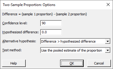
-
Press OKOK and OKOK.
Test and CI for Two Proportions
Method
p1: proportion where Sample 1 = Event p2: proportion where Sample 2 = Event Difference: p1 - p2 Descriptive Statistics
Sample N Event Sample p Sample 1 72 10 0.138889 Sample 2 72 8 0.111111 Estimation for Difference
Difference 90% Lower
Bound for
Difference0.0277778 -0.042799 CI based on normal approximation Test
Null hypothesis H0: p1 − p2 = 0 Alternative hypothesis H1: p1 - p2 > 0 Method Z-Value P-Value Normal approximation 0.50 0.307 Fisher's exact 0.401 The test based on the normal approximation
uses the pooled estimate of the proportion (0.125).
Two Sample t-Test (Independent Samples)
Using Data:
-
Enter the data for the first sample into column C1C1 and the second sample into column C2C2.
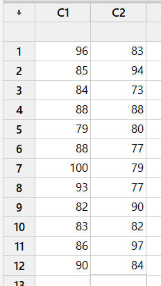
-
Choose StatStat, Basic StatisticsBasic Statistics, and 2-Sample tTwo Sample t.
-
From the dropdown choose Each sample is in its own columnEach sample is in its own column. Select "C1" for Sample 1:Sample One colon and "C2" for Sample 2:Sample Two colon
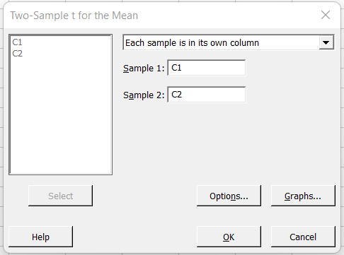
-
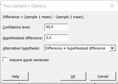
Select OptionsOptions to set the appropriate Confidence Level:Confidence Level colon, Hypothesized differenceHypothesized difference, and Alternative hypothesisAlternative hypothesis. Check box if we Assume equal variancesAssume equal variances. Press OKOK.
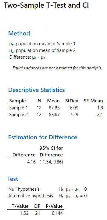
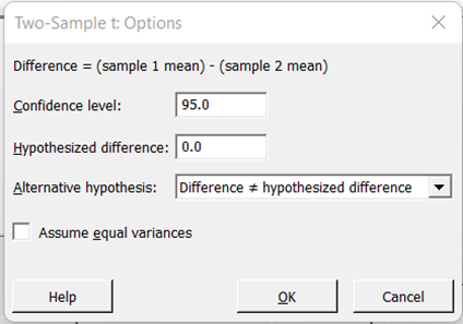
-
Press OKOK.
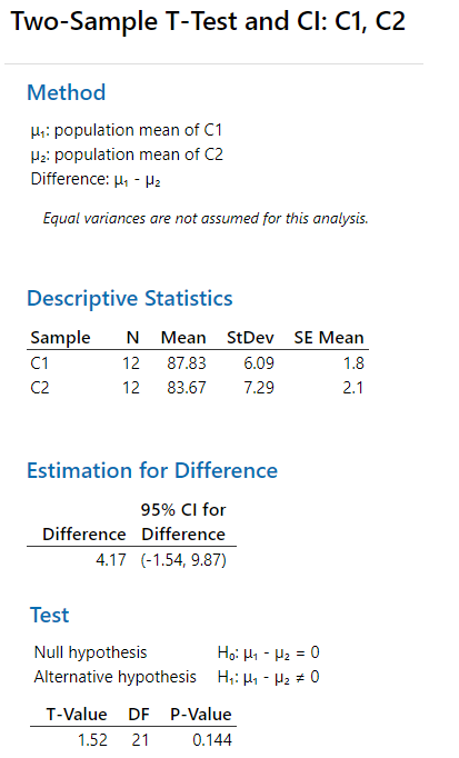
Using Summary Statistics:
-
Choose StatStat, Basic StatisticsBasic Statistics, and 2-Sample tTwo Sample t.
-
From the dropdown choose Summarized dataSummarized data. Enter the Sample sizeSample size, Sample meanSample mean, and the Standard deviationStandard deviation for each sample.
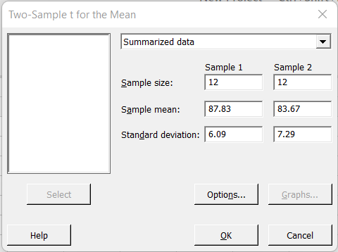
-
Select OptionsOptions to set the appropriate Confidence Level:Confidence Level colon, Hypothesized differenceHypothesized difference, and Alternative hypothesisAlternative hypothesis. Check box if we Assume equal variancesAssume equal variances. Press OKOK.
-
Press OKOK.
Two Sample t-Test (Dependent Samples, Paired Difference)
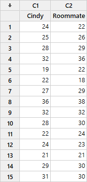
Method: Raw Data
-
Enter the data for the first sample into C1 and the second sample into C2.
-
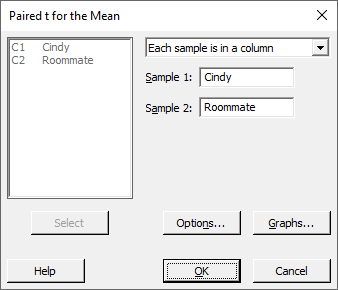
Select StatStat, Basic StatisticsBasic Statistics, Paired tPaired t
-
From the dropdown choose Each sample is in a columnEach sample is in a column.
-
Click the mouse in the box labeled Sample 1Sample One. Highlight the appropriate column in the box on the left. Press SelectSelect. Click the mouse in the box labeled Sample 2Sample Two, highlight the appropriate column in the box on the left, and press SelectSelect.
Note that Minitab calculates the paired differences by subtracting the values for the second sample from the values for the first sample, which is the opposite of what we do when we calculate them by hand or using a TI-83/84 Plus calculator.
-
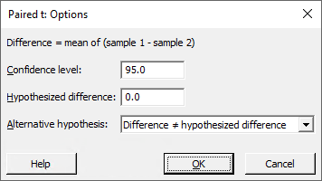
Choose OptionsOptions to adjust the Confidence levelConfidence level, Hypothesized differenceHypothesized difference, and Alternative hypothesisAlternative hypothesis.
-
Press OKOK and OKOK.
Paired T-Test and CI: Cindy, Roommate
Descriptive Statistics
Sample N Mean StDev SE Mean Cindy 15 26.67 4.81 1.24 Roommate 15 27.33 5.69 1.47 Estimation for Paired Difference
Mean StDev SE Mean 95% CI
for μ_difference-0.667 2.059 0.532 (-1.807, 0.473) µ_difference: mean of (Cindy - Roommate) Test
Null hypothesis H0: μ_difference = 0 Alternative hypothesis H1: μ_difference ≠ 0 T-Value P-Value -1.25 0.230
Two Sample F-Test
-
Select StatStat, Basic StatisticsBasic Statistics, 2 VariancesTwo Variances.
-
From the dropdown choose Sample variancesSample variances.
-
Enter the Sample sizeSample size and the VarianceVariance for each sample.
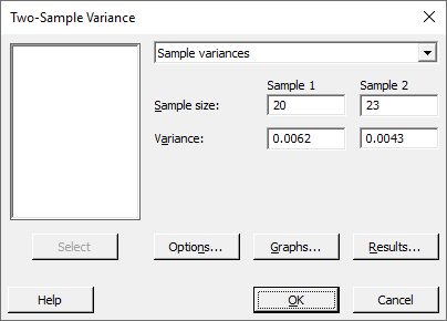
-
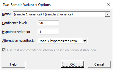
Press OptionsOptions. For the RatioRatio dropdown choose (sample 1 variance) / (sample 2 variance)left parenthesis sample One variance right parenthesis divided by right parenthesis sample Two variance right parenthesis. Enter a Confidence levelConfidence level, Hypothesized ratioHypothesized ratio (default is 1), and Alternative hypothesisAlternative hypothesis.
-
Press OKOK and OKOK.
Test and CI for Two Variances
Method
σ12: variance of Sample 1 σ22: variance of Sample 2 Ratio: σ12/σ22 F method was used. This method is accurate for normal data only. Descriptive Statistics
Sample N StDev Variance 90% Lower
Bound for
σ2Sample 1 20 0.079 0.006 0.004 Sample 2 23 0.066 0.004 0.003 Ratio of Variances
Estimated
Ratio90% Lower
Bound for
Ratio
using F1.44186 0.816 Test
Null hypothesis H2: σ12 / σ₂2 = 1 Alternative hypothesis H1: σ12 / σ₂2 > 1 Significance level α = 0.1 Method Test
StatisticDF1 DF2 P-Value F 1.44 19 22 0.204
Nonparametrics
The Kruskal-Wallis Test
-
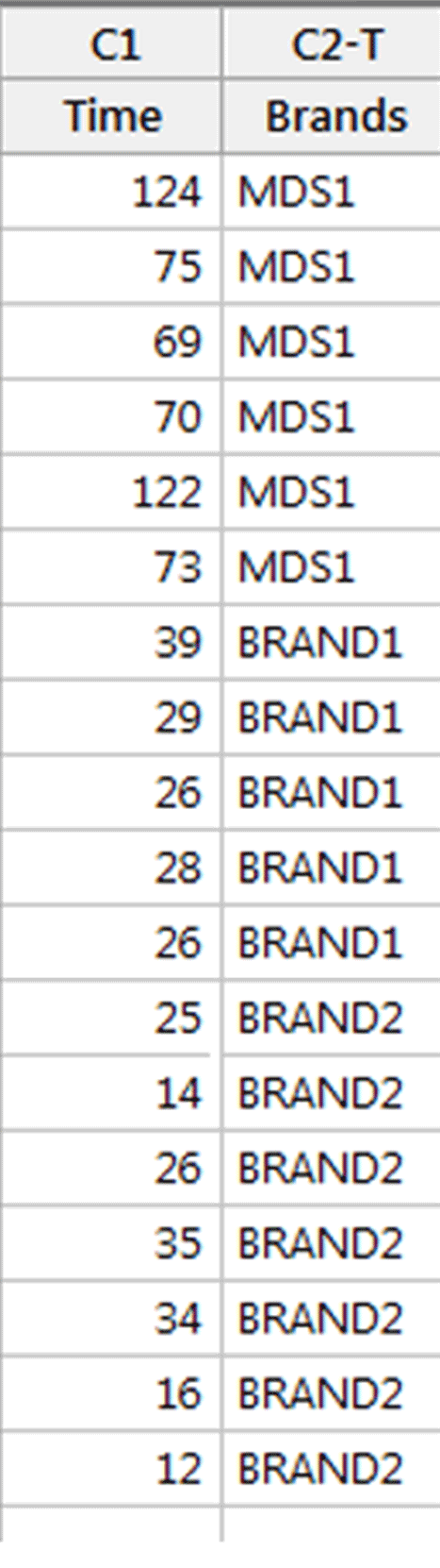
Enter the category labels in Column C2Column C2. Enter the corresponding data value in Column C1Column C1.
-
Choose StatStat, NonparametricsNonparametrics, and Kruskal-WallisKruskal minus Wallis.
-
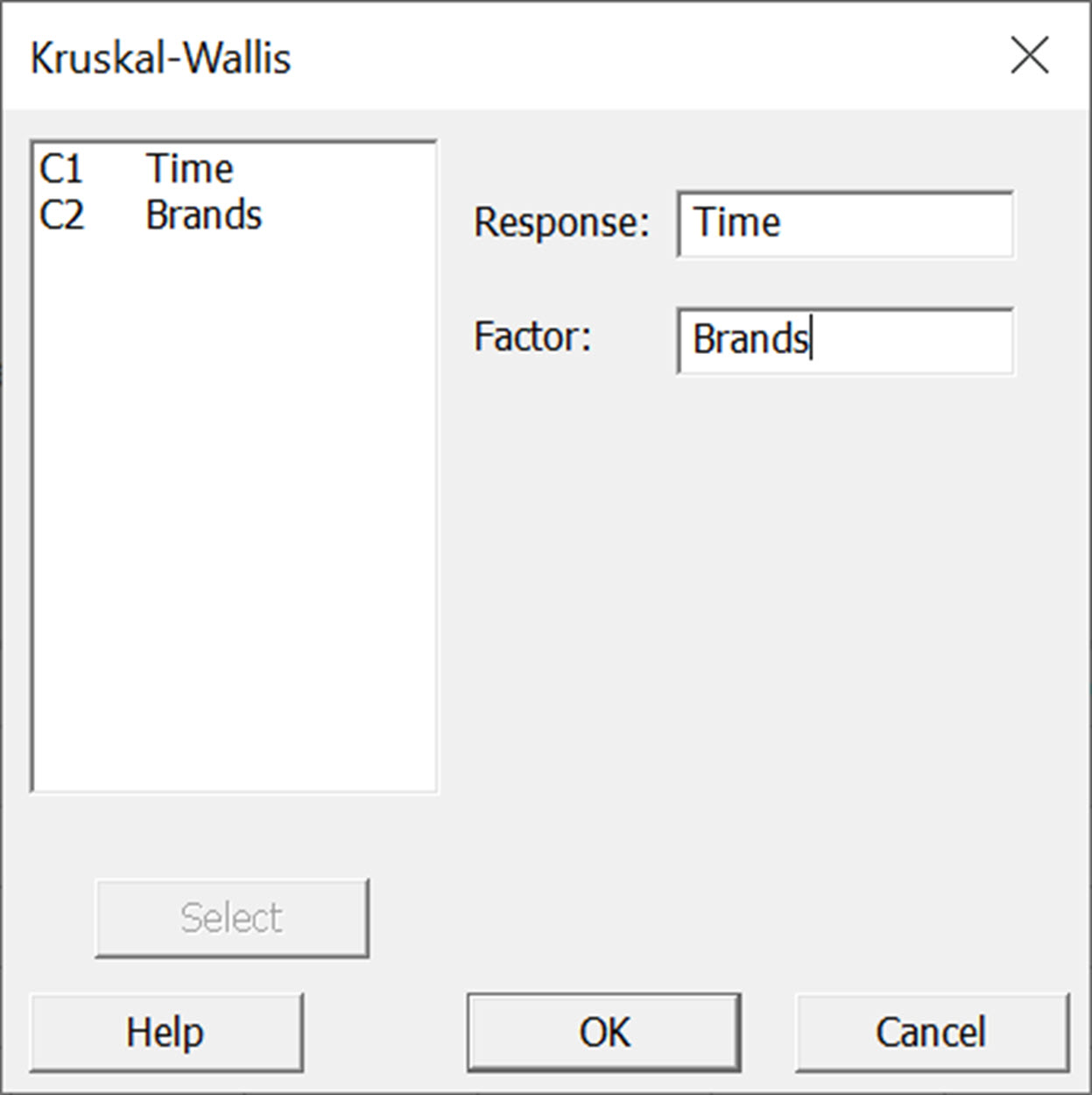
Enter the data for the ResponseResponse and the categories for the FactorFactor. Press OKOK.
-
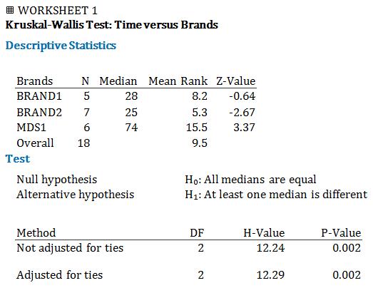
Observe the results of the Kruskal-Wallis Test.
Runs Test for Randomness
-
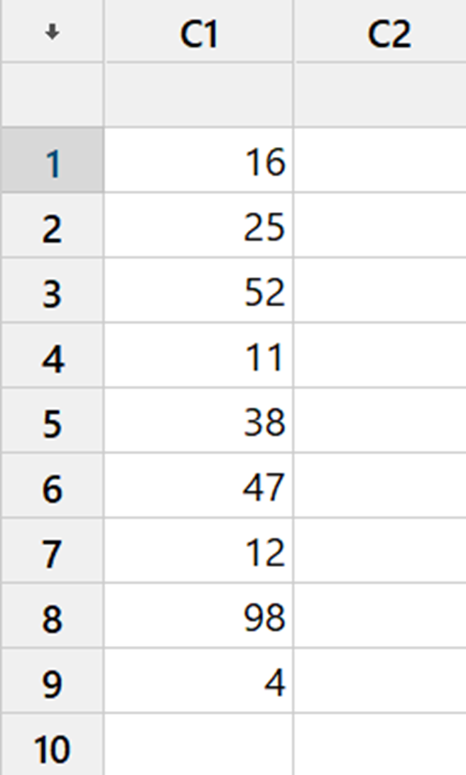
Enter the data into column C1C1.
-
Choose StatStat, NonparametricsNonparametrics, and Runs TestRuns Test.
-
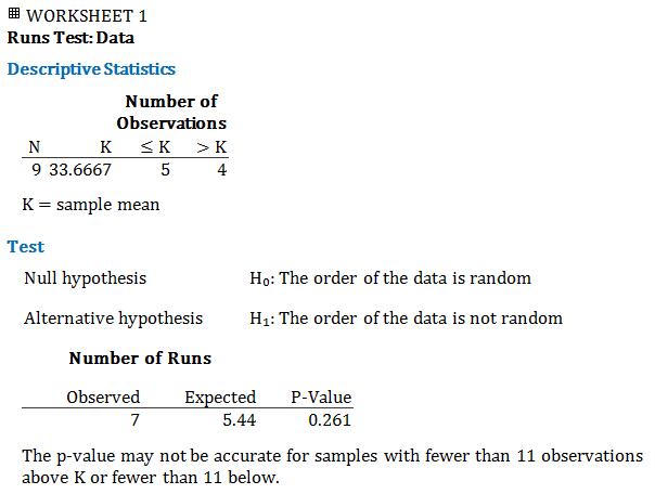
Select C1C1 as the variables. Press OKOK.
-
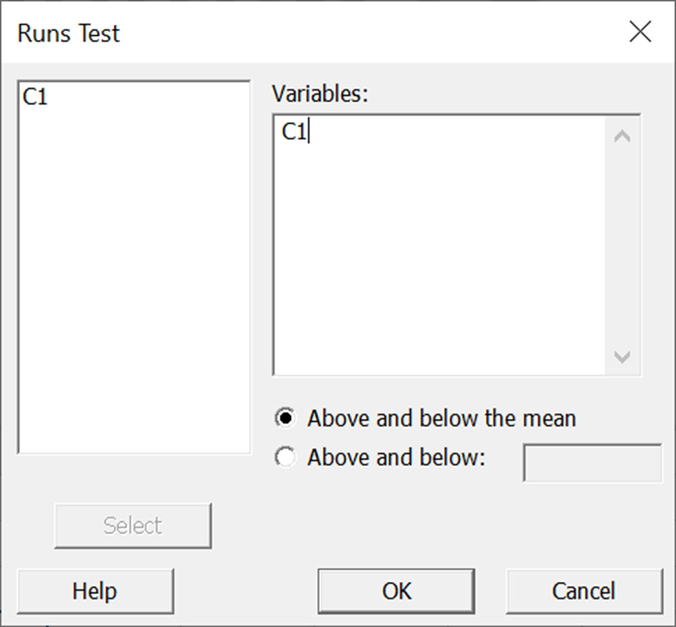
Observe the outcome of the runs test.
Sign Test
-
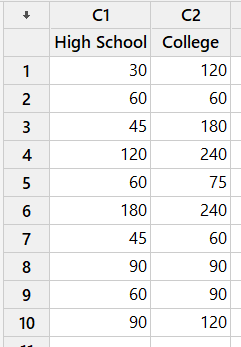
Enter the category labels in Column C1C1. Enter the corresponding data value in Column C2C2.
-
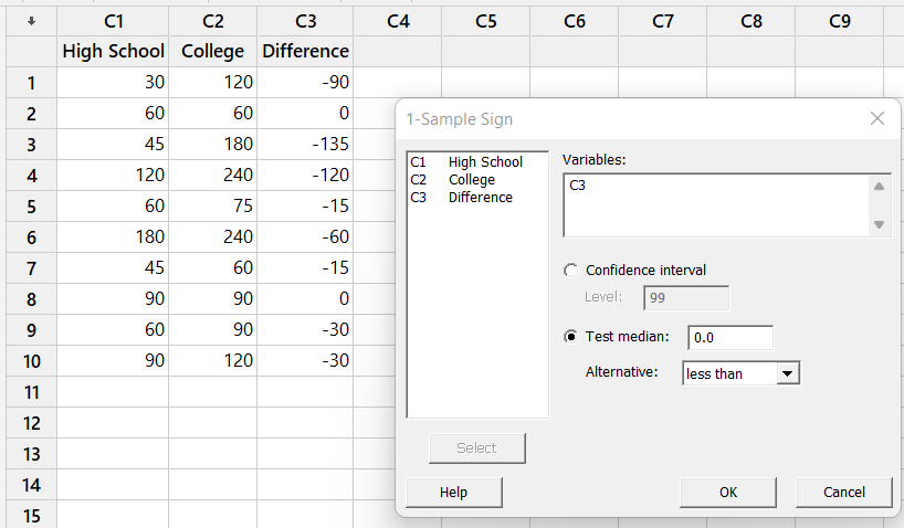
Choose ViewView, and then Command Line/HistoryCommand Line divided by History. In the Command Line box enter Let C3=C1-C2Let c3 equals C1 minus C2. Press RunRun. The differences are now calculated in column C3.
-
Choose StatStat, NonparametricsNonparametrics and 1-Sample SignOne Sample Sign.
-
Enter C3C3 for VariablesVariables and select the radio button next to Test medianTest median. Choose the appropriate AlternativeAlternative from the drop down and press OKOK.
-
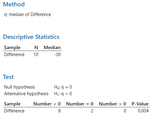
Observe the results of the test.
Spearman Rank Correlation Test
-
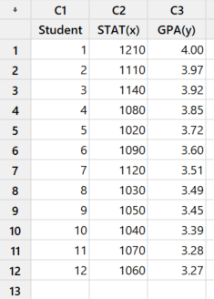
Enter data in different columns.
-
Choose StatStat, Basic StatisticsBasic Statistics, and CorrelationCorrelation.
-
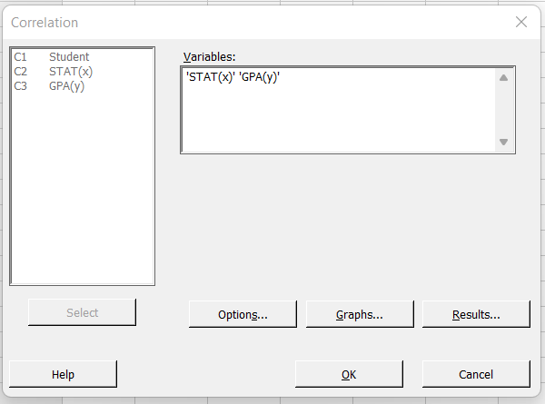
Enter the desired columns for the two associated variables in the VariablesVariables box. Select OptionsOptions and select Spearman correlationSpearman correlation from the MethodMethod drop down menu and input the desired Confidence levelConfidence level. Press OKOK. Press OKOK again.
-
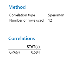
Observe the results.
Wilcoxon Rank-Sum Test
-
Input the data into Columns C1 and C2.
-
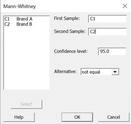
Choose Stat, Nonparametrics, and Mann-Whitney. Enter C1 as the First Sample and C2 as the Second Sample. Enter the desired confidence level and Alternative hypothesis. Press OK.
-
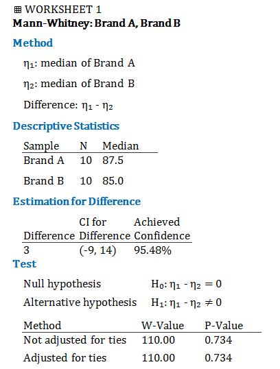
Observe the result of the Wilcoxon rank-sum test (also known as the Mann-Whitney test).
Wilcoxon Signed-Rank Test
-
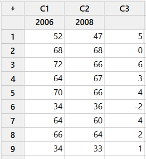
Enter the data into Column C1C1 and Column C2C2.
-
Choose ViewView, and then Command Line/HistoryCommand Line divided by History.
-
In the Command LineCommand Line box, enter Let C3=C1-C2Let c3 equals C1 minus C2. Press RunRun. The differences are now calculated in column C3C3.
-
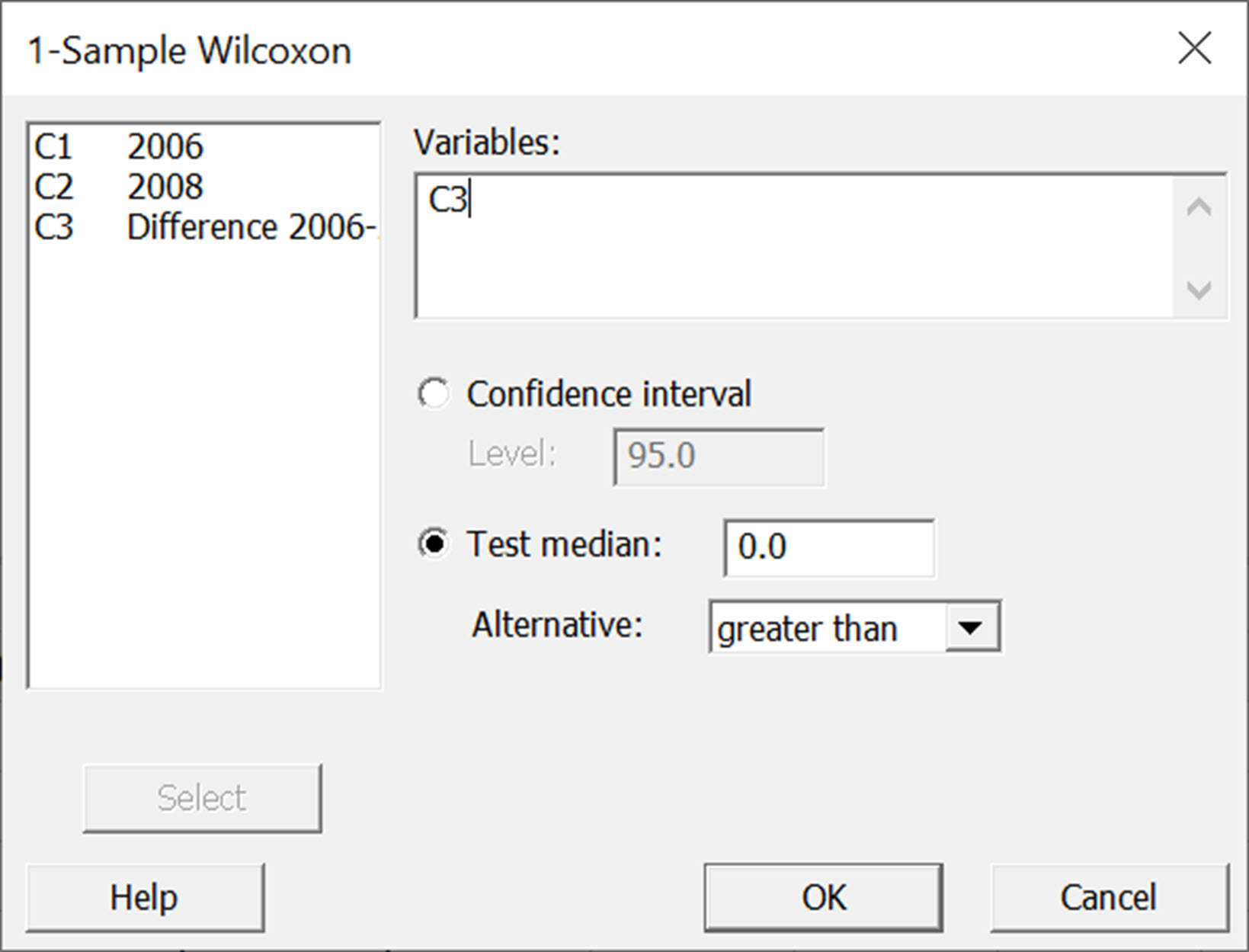
Choose StatStat, NonparametricsNonparametrics and 1-Sample WilcoxonOne Simple Wilcoxon.
-
Enter C3C3 for variables and select the radio button next to Test medianTest median. Choose the appropriate AlternativeAlternative from the drop down and press OKOK.
-
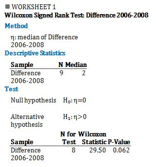
Observe the output screen for the Wilcoxon signed-rank test.
Normal Distribution
Inverse Normal
-
To find a z- or x-value for a given probability in Minitab, enter the probability in the first column and row.
-
Go to Calc > Probability Distributions > Normal.
-
When the Normal Distribution menu appears, select Inverse cumulative probability and enter the Mean and Standard deviation.
-
Select C1 as the Input column. Click OKOK, and the probability will appear in the Session window.
Note: The probability is the area under the normal distribution curve to the left of the z-score or x-value calculated by Minitab.
Normal Probability (cdf)
-
Enter the given x- or z-value in the first column and row.
-
Go to Calc > Probability Distributions > Normal.
-
When the Normal Distribution menu appears, make sure Cumulative probability is selected and enter the Mean and Standard deviation.
-
Select C1 as the Input column. Once you are finished, click OKOK, and the probability will appear in the Session window.
Note: Minitab only calculates the area under the normal distribution curve to the left of the given z-score or x-value.
Test for Normality
-
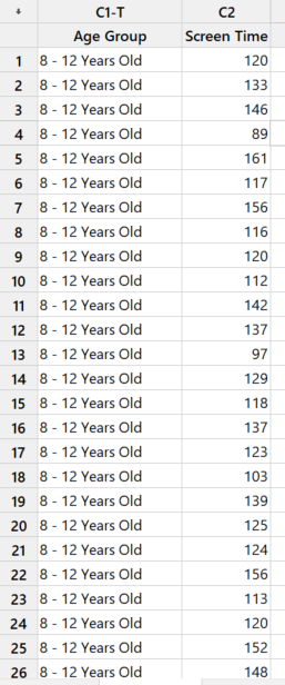
Enter the category labels in Column C1C1. Enter the corresponding data value in Column C2C2.
-
Choose StatStat, Basic StatisticsBasic Statistics, and Normality TestNormality Test.
-
Enter the data for the variable. Select the desired Test for NormalityTest for Normality. Press OKOK.
-
Observe the results of the Test for Normality.
Poisson Distribution
Poisson Probability Distribution
-
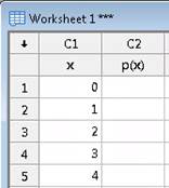
Set up the worksheet with "x" as the label for the first column, C1 and "p(x)" as the label for C2. In C1C1 starting with row 1, enter whole numbers for the value of the discrete random variable.
-
Press CalcCalc, ProbabilityProbability DistributionsDistributions, and PoissonPoisson.
-
Designate ProbabilityProbability for the pdfpdf. (Alternatively, Cumulative ProbabilityCumulative Probability for the cdfcdf.)
-
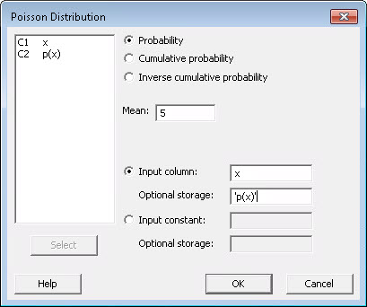
Complete the dialog box by inputting "5" for the MeanMean, selecting "x" for the Input columnInput column and selecting "p(x)" for Optional storageOptional storage.
-
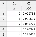
Press OKOK and the Poisson probabilities are displayed in column C2.
Regression
Confidence Intervals for Slope and y-Intercept
-
Enter your X and Y data into two columns, C1 and C2.
-
Press StatStat, RegressionRegression, and RegressionRegression, then Fit Regression ModelFit Regression Model.
-
Enter the Response variable and the Predictor variable (continuous).
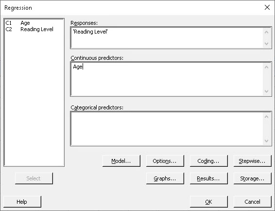
-
Click ResultsResults and then choose Display of resultsDisplay of results: Expanded tables. Click OKOK and OKOK.
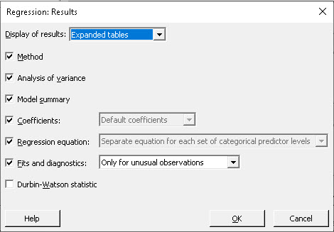
-
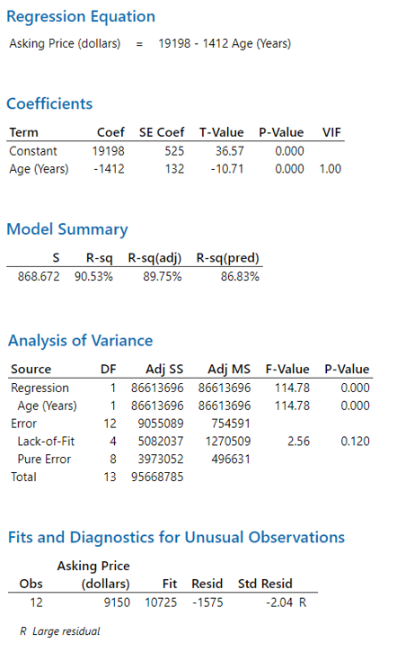
Note in the following example that the confidence intervals for the slope (Constant) and y-intercept (Age) are displayed in the output under the Coefficients heading.
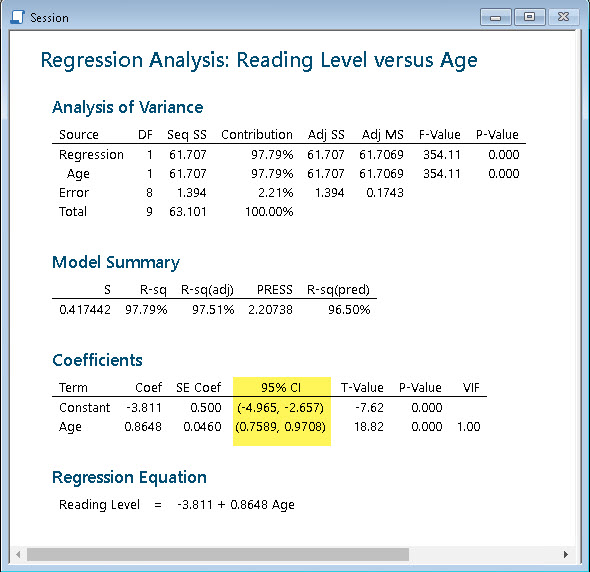
Linear Regression Fitted Line Plot with Confidence Interval
-
Enter your data in the worksheet.
-
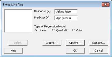
Under the Stat menu select RegressionRegression, and Fitted Line PlotFitted Line Plot.
-
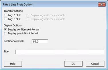
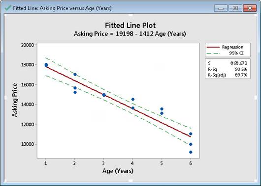
Select the Response (Y)Response left parenthesis Y right parenthesis and Predictor (X)Predictor left parenthesis X right parenthesis, make sure the Type of Regression Model is Linear. Click OptionsOptions and under Display OptionsDisplay Options check Display confidence intervalDisplay confidence interval. Click OKOK and OKOK.
Linear Regression Fitted Line Plot with Prediction Interval
-
Enter your data in the worksheet.
-
Under the Stat menu select RegressionRegression, and Fitted Line PlotFitted Line Plot.
-
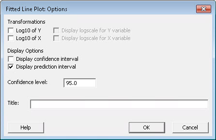
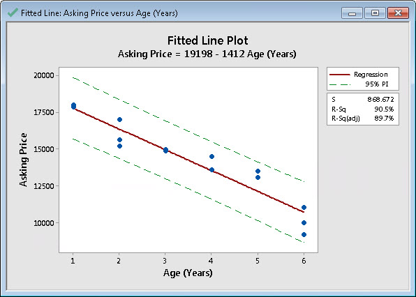
Select the Response (Y)Response left parenthesis Y right parenthesis and Predictor (X)Predictor left parenthesis X right parenthesis, make sure the Type of Regression Model is Linear. Click OptionsOptions and under Display OptionsDisplay Options check Display prediction intervalDisplay prediction interval. Click OKOK and OKOK.
Multiple Regression
-
Enter the data in columns with the variable names at the top of each column.
-
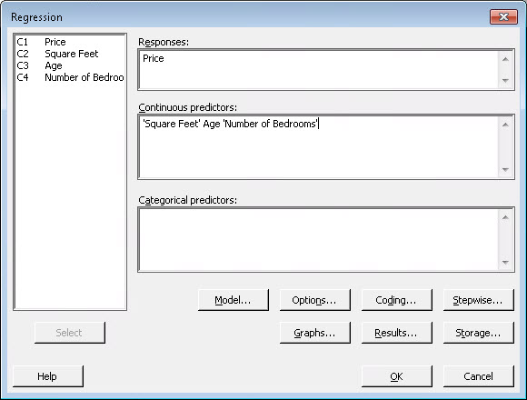
Under Stat, choose RegressionRegression, then RegressionRegression, and Fit Regression Model…Fit Regression Model horizontal ellipse.
-
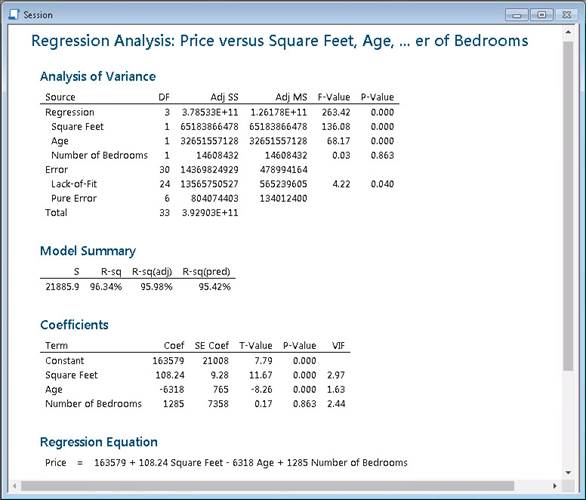
In the dialog box, use SelectSelect to input the Reponse variable and the Predictor variables. Select OKOK.
Regression Prediction Intervals
-
Enter the data in columns with the variable names at the top of each column.
-
First run Regression (see Linear Regression or Multiple Regression).
-
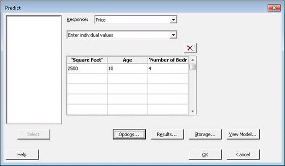
Under Stat, choose RegressionRegression, then RegressionRegression, and PredictPredict
-
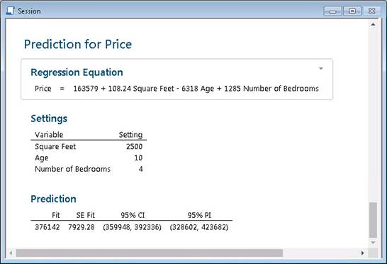
Enter the individual value(s) you wish to predict for. Use Options…Options… to select the Confidence Level. Select OKOK and OKOK.
Simple Linear Regression
-
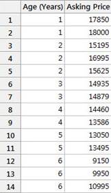
Enter your X and Y data into two columns, C1 and C2.
-
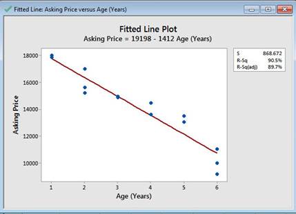
Press StatStat, RegressionRegression, andFitted Line PlotFitted Line Plot. Enter the Response variable and the Predictor variable, and press OKOK.
-
Observe the least squares coefficients, , and standard error, as well as the regression plot.
-
Press StatStat, RegressionRegression, and RegressionRegression, then Fit Regression ModelFit Regression Model for additional output. Enter the Response variable and the Predictor variable (continuous), and press OKOK.
Sampling
Random Samples
-
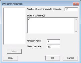
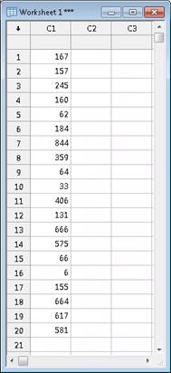
Press CalcCalc, and select Random DataRandom Data, and then choose IntegerInteger.
-
Complete the dialog box with Number of rows of data to generate, Store in column(s), Minimum value, and Maximum value.
-
Observe the random numbers.
t-Distribution
Inverse t
-
Enter the area to the left of the desired t-value in the first row of column C1. If the area we are given is to the right of the t-value, we must first determine the area to the left by calculating (1-area to the right).
-
Go to CalcCalc,Probability DistributionsProbability Distributions, tt.
-
Select Inverse cumulative probabilityInverse cumulative probability and enter the number of degrees of freedom. Select C1 as the input column.
-
Click OKOK and the t-value will appear in the Session window.
Time Series
Simple Exponential Smoothing
-
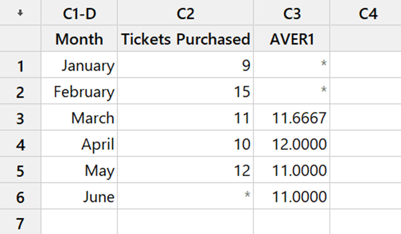
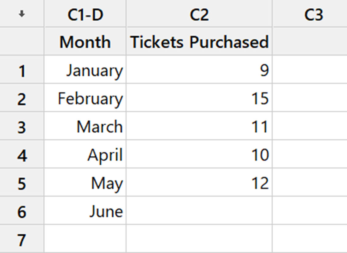
Enter the data of the table into the Minitab worksheet. Make sure the cell for the period you are trying to forecast is blank (the *asterisk times sign is not blank). To remove the *asterisk times sign, right click on the cell and select Clear CellsClear Cells.
-
Choose StatStat, Time SeriesTime Series, and Single Exp SmoothingSingle Exp Smoothing.
-
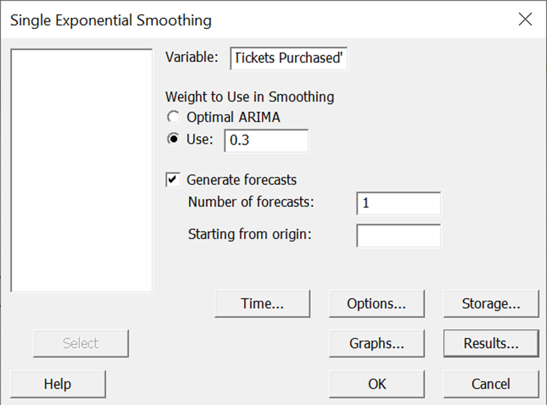
Enter C2C2 in the VariableVariable box. Under Weight to Use in SmoothingWeight to use Use in Smoothing, select the radio button next to Use and enter the desired alpha level. Check the box for Generate forecastsGenerate forecasts and enter the Number of forecastsNumber of forecasts (using a value of 1 will give the first forecast). Click on OptionsOptions and enter 1one for KK. Press OKOK. Click on StorageStorage and check the box for ForecastsForecasts. Press OKOK. Click on Results and check the box for Summary table and results tableSummary table and results table. Press OKOK. Press OKOK again.
-
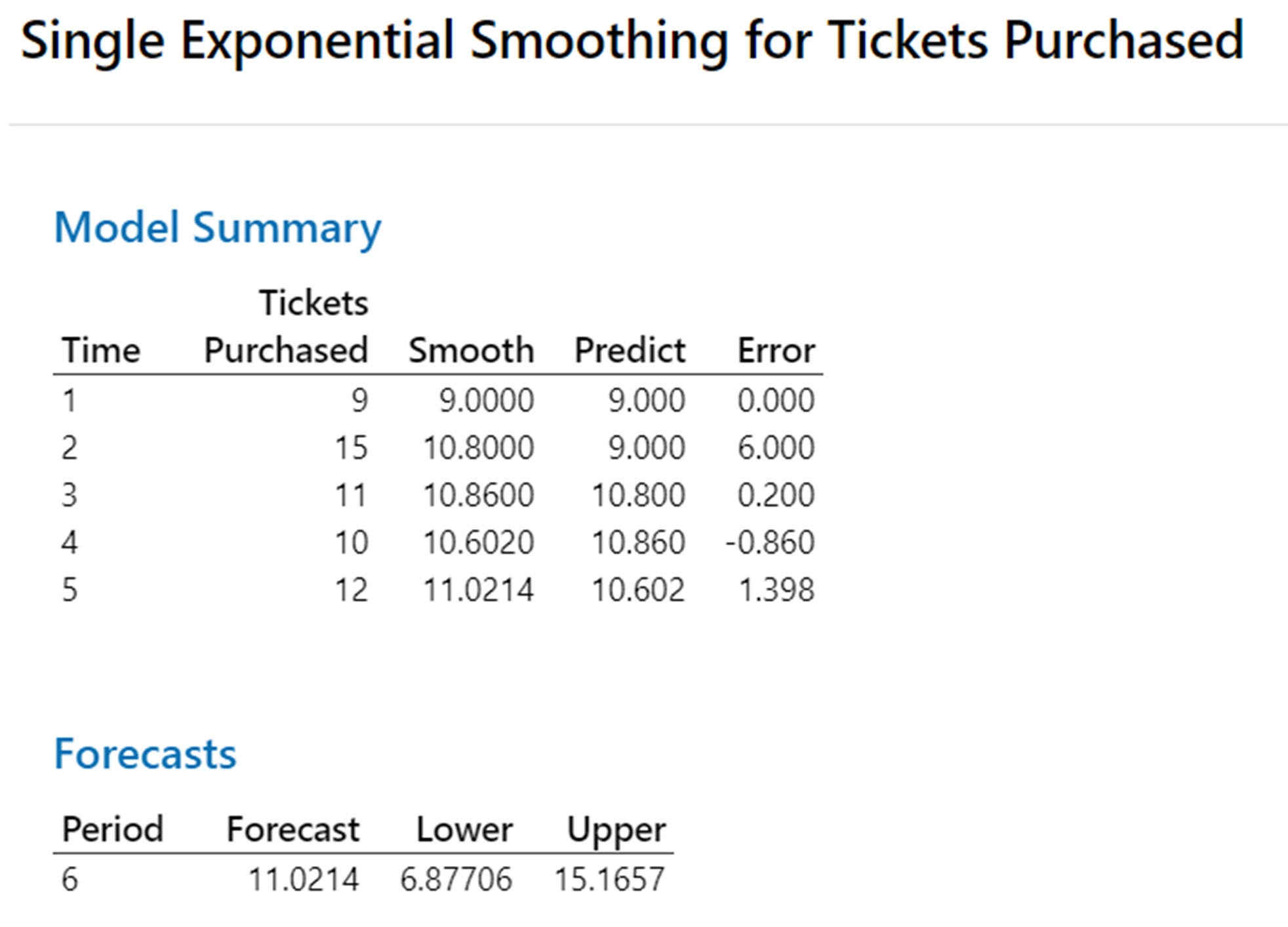
Observe the results.
Simple Moving Average
-
Enter the data into the Minitab worksheet.
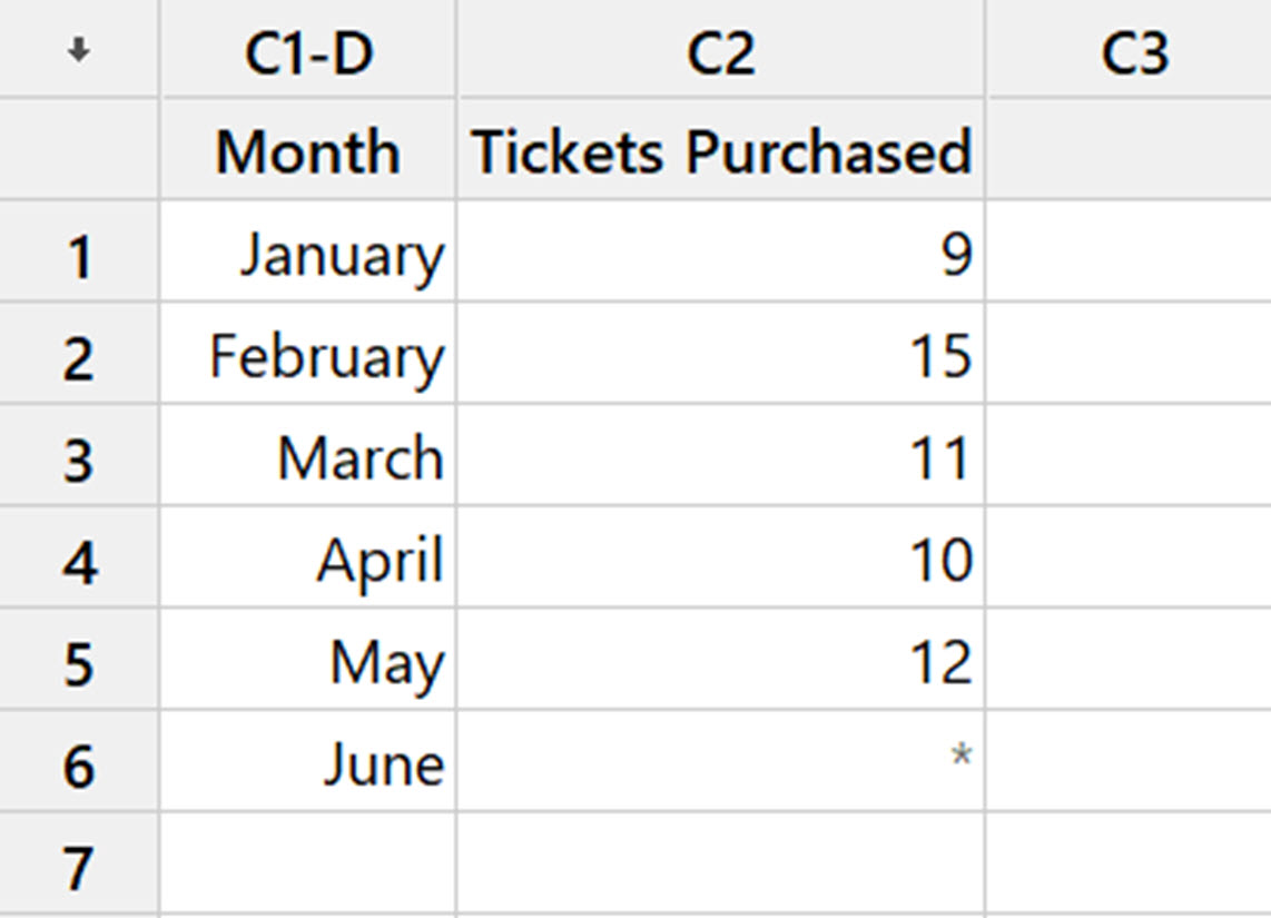
-
Choose StatStat, Time SeriesTime Series, and Moving AverageMoving Average.
-
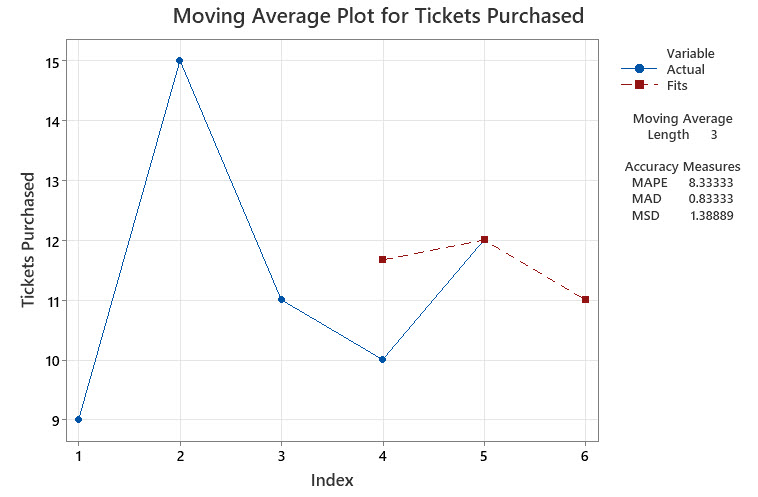
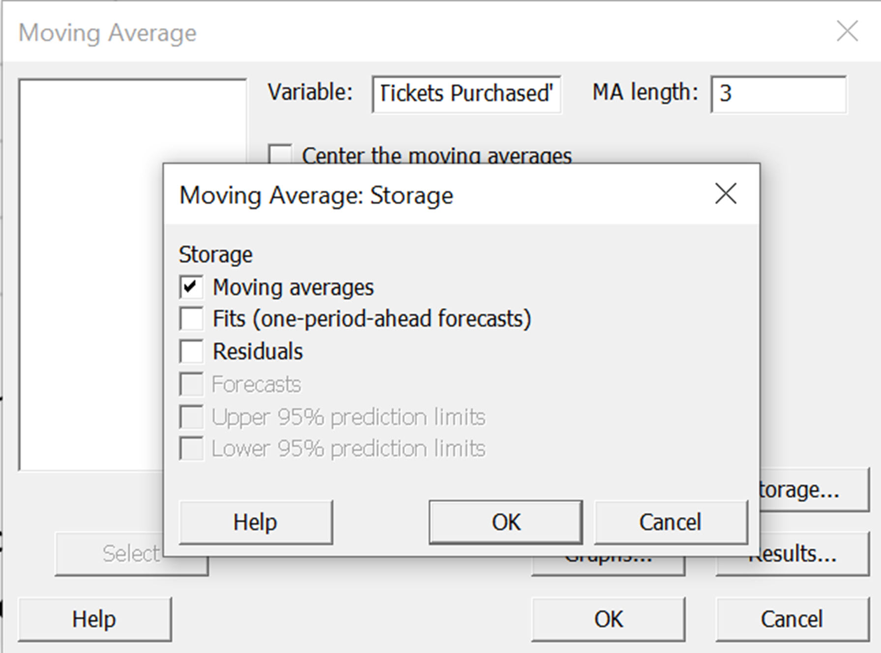
Enter C2C2 in the VariableVariable box, and nn, the number of periods, in the MA lengthMA length box. Click on StorageStorage and check the box for Moving AveragesMoving Averages. Press OKOK. Press OKOK again.
-
Observe the results.