TI-89 Calculator
Graphing a Function
-
Press ◆◆ semicolon, then F1F1 to open the Y= editor.
-
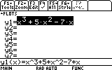
Input the function, with x as the variable.
-
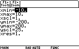
Press ◆◆ semicolon, then F2F2 to input window settings.
-
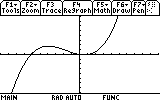
Press ◆◆ semicolon, then F3F3 to display the graph.
-
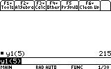
To evaluate the function you input into the y1=y1 equals field of the Y= editor at a given value of x, first press HOMEHome to display the home screen. Input y1(Y1 left parenthesis, then the given value of x, and then a right parenthesis. Then press ENTERthe Enter key.
Graphing a Piecewise Defined Function with Two Pieces
-
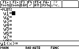
Press ◆◆ semicolon, then F1F1 to open the Y= editor.
-
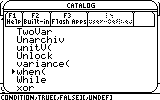
Press CATALOGCatalog, then .dot to select when(when left parethesis.
-
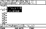
Press ENTERthe Enter key. Using x as the variable, input the domain of the first function as an inequality, then a comma, input the first function, then a comma, input the second function, and then input a right parenthesis.
-
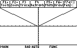
Press ◆◆ semicolon, then F3F3 to display the graph.
Graphing a Piecewise Defined Function with Three Pieces
-
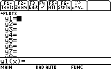
Press ◆◆ semicolon, then F1F1 to open the Y= editor.
-
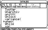
Press CATALOGCatalog, then .dot to select when(when left parethesis.
-
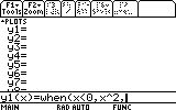
Press ENTERthe Enter key. Using x as the variable, input the domain of the first function as an inequality, then a comma, input the first function, then another comma.
-
Press CATALOGCatalog, then .dot to select when(when left parethesis, and then press ENTERthe Enter key.
-
Input the domain of the second function as an inequality, then a comma, input the second function, then a comma, input the third function, and then input two right parentheses (one for each when(when left parenthesis function).
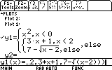
-
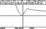
Press ◆◆ semicolon, then F3F3 to display the graph.
Graphing: Setting Window Parameters
-
Press ◆◆ semicolon, then F1F1 to open the Y= editor.
-
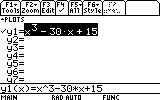
Input the function, with x as the variable.
-
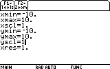
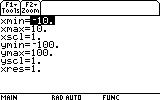
Press ◆◆ semicolon, then F2F2 to input window settings.
-
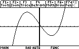
Press ◆◆ semicolon, then F3F3 to display the graph.
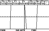
-
If necessary, repeat Step 3 to adjust the window settings to get a better view of the graph and then repeat Step 4 to display the graph.
Graphing: Zooming In
-
Press ◆◆ semicolon, then F1F1 to open the Y= editor.
-
Input the function or functions that you wish to graph, with x as the variable.
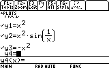
-
Press ◆◆ semicolon, then F2F2 to input window settings.
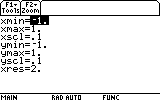
-
Press ◆◆ semicolon, then F3F3 to display the graph.
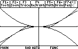
-
Press F2F2 to open the Zoomzoom menu and scroll down to 2:ZoomInTwo colon zoom in.
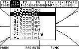
-
Press ENTERthe Enter key as many times as desired to zoom in on graph.
-
Press ◆◆ semicolon, then F3F3 to display the graph.
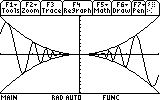
Graphing: Improving Appearance
-
Press ◆◆ semicolon, then F1F1 to open the Y= editor.
-
Input the function, with x as the variable.
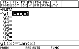
-
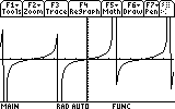
Press ◆◆ semicolon, then F3F3 to display the graph.
-
To improve the appearance of the graph, first press ◆◆ semicolon, then F1F1 to open the Y= editor.
-
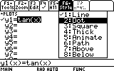
Press 2ndsecond, then F1F1 to open the Stylestyle menu. Scroll down to 2:Dot2 colon dot and press ENTERthe Enter key.
-
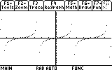
Press ◆◆ semicolon, then F3F3 to display the graph.
Least-Squares Curve Fitting
-
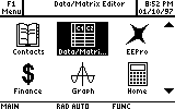
Press APPSApplications, then scroll to Data/Matrix Editordata divided by Matrix Editor.
-
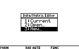
Press ENTERthe Enter key. Scroll down to 3:NewThree colon new.
-
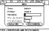
Press ENTERthe Enter key. Scroll down to the Variablevariable: field, and input a name for the new data variable (for example, c).
-
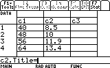
Press ENTERthe Enter key twice. Input the values of the independent variable in column c1c1, and input the corresponding values of the dependent variable in column c2c2.
-
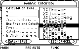
Press F5F5. Press ►► semicolon to select a Calculation TypeCalculation Type and scroll down to 5:LinReg5 colon linereg.
-
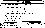
Press ENTERthe Enter key twice. Input c1c1 in the xx field and c2c2 in the yy field.
-
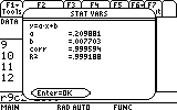
Press ENTERthe Enter key to calculate the slope aa and y-intercept bb of the best-fitting line for the data.
Visualizing Limits
-
Press ◆◆ semicolon, then F1F1 to open the Y= editor.
-
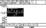
Input the function whose limit you wish to visualize, with x as the variable.
-
Press ◆◆ semicolon, then F2F2 to input window settings. Be sure the interval of x-values for the viewing window includes the value that the independent variable approaches in the limit.
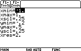
-
Press ◆◆ semicolon, then F3F3 to display the graph.
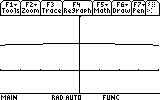
-
Press ◆◆ semicolon, then F2F2 to input new window settings.
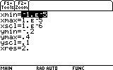
-
Press ◆◆ semicolon, then F3F3 to display the graph in the new viewing window. Use caution when trying to determine the value of a limit by inspecting graphs of a function. This may or may not lead to a correct guess for the limit, depending on the viewing window specified for each graph.
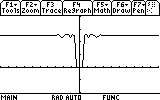
Predicting Limits
-
Press ◆◆ semicolon, then F1F1 to open the Y= editor.
-
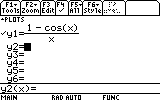
Input the function whose limit you wish to predict, with x as the variable.
-
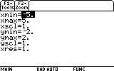
Press ◆◆ semicolon, then F2F2 to input the window settings.
-
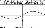
Press ◆◆ semicolon, then F3F3 to display the graph.
-
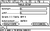
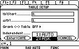
Press ◆◆ semicolon, then F4F4 to display the TABLE SETUPTABLE SETUP dialog box.
-
Scroll down to the Independentindependent field. Press ►► semicolon and scroll to down to 2:ASK2 colon ask. Press ENTERthe Enter key.
-
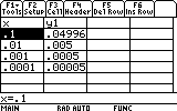
Press ◆◆ semicolon, then F5F5 to display the table. Input values in the xx column that approach the value that the independent variable approaches in the limit. The calculator will generate corresponding values of the function in the y1y1
Finding Roots of an Equation of the Form f(x)=0
-
Press ◆◆ semicolon, then F1F1 to open the Y= editor.
-
Input the function, with x as the variable.
 = 0_1 - FUNCTION ENTERED.png)
-
Press ◆◆ semicolon, then F2F2 to input the window settings.
 = 0_2 - WINDOW SETTINGS.png)
-
Press ◆◆ semicolon, then F3F3 to display the graph.
 = 0_3 - GRAPH.png)
-
Press F5F5 to open the MathMath menu, and scroll down to 2:Zero2 colon Zero.
 = 0_4 - MATH MENU.png)
-
Press ENTERthe Enter key.
 = 0_5 - GRAPH WITH CURSOR.png)
-
Press ◄◄ semicolon as many times as desired to move to any position to the left of the desired root, which is an x-intercept on the graph. This is the lower bound of the interval for x.
 = 0_6 - ESTABLISHING LOWER BOUND.png)
-
Press ENTERthe Enter key to set the lower bound chosen in Step 7.
-
Press ►► semicolon as many times as desired to move to any position to the right of the desired root. This is the upper bound of the interval for x.
 = 0_7 - ESTABLISHING UPPER BOUND.png)
-
Press ENTERthe Enter key to set the upper bound chosen in Step 9. The calculator will display the root of the equation that occurs within the specified interval for x.
 = 0_8 - FINAL RESULT.png)
Evaluating a Definite Integral
-
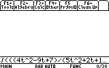
From the calculator Home screen, press 2ndsecond, then 7Seven to input ∫(integral left parenthesis.
-
Input the integrand function, then a comma, input the variable of integration, then a comma, input the lower limit of integration, then a comma, input the upper limit of integration, and then input a right parenthesis.
-
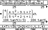
Press ENTERthe Enter key to evaluate the integral.
Graphing Parametrically Defined Curves
-
Press MODEmode, select the GraphGraph field, and press ►► semicolon.
-
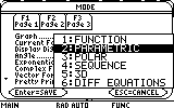
Scroll down to 2:PARAMETRIC2 colon PARAMETRIC and press ENTERthe Enter key.
-
If necessary, change the AngleAngle mode to the units (RADIANRADIAN or DEGREEDEGREE) you want to use for t.
-
Press ENTERthe Enter key again to save the settings and exit the MODEMODE dialog box.
-
Press ◆◆ semicolon, then F1F1 to open the Y= editor.
-
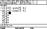
Input the desired parametrized formulas for x and y into the xt1xt1 and yt1yt1 fields, respectively, with t as the variable.
-
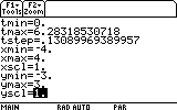
Press ◆◆ semicolon, then F2F2 to input window settings.
-
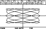
Press ◆◆ semicolon, then F3F3 to display the graph.
-
When you are finished graphing parametrically defined curves, press MODEmode and set the GraphGraph mode back to 1:FUNCTION1 colon FUNCTION.
Graphing Polar Equations
-
Press MODEmode, select the GraphGraph field, and press ► ► semicolon.
-
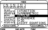
Scroll down to 3:POLAR3 colon POLAR and press ENTERthe Enter key.
-
If necessary, change the AngleAngle mode to the units (RADIANRADIAN or DEGREEDEGREE) you want to use for θ.
-
Press ENTERthe Enter key again to save the settings and exit the MODEMODE dialog box.
-
Press ◆◆ semicolon, then F1F1 to open the Y= editor.
-
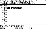
Input the expression for r, with θ as the variable.
-
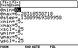
Press ◆◆ semicolon, then F2F2 to input window settings.
-
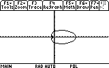
Press ◆◆ semicolon, then F3F3 to display the graph.
-
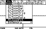
Press F2F2 to open the Zoomzoom menu, and scroll down to A:ZoomFitA colon ZoomFit.
-
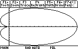
Press ENTERthe Enter key.
-
When you are finished graphing polar equations, press MODEmode and set the GraphGraph mode back to 1:FUNCTIONOne colon FUNCTION.
Graphing Conic Sections in Cartesian Coordinates
-
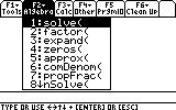
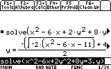
From the calculator Home screen, press F2F2, then ENTERthe Enter key to input solve(solve left parenthesis.
-
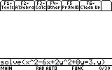
Input the Cartesian equation of the conic section, then a comma, then yy, and then a right parenthesis.
-
Press ENTERthe Enter key.
-
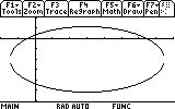
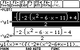
Press ◆◆ semicolon, then F1F1 to open the Y= editor. Input the two solutions found in Step 3 into the y1=y1 equals and y2=y2 equals fields. (Note that if the conic section is a parabola that opens up or down, then there will be only one solution to input into the y1=y1 equals field.)
-
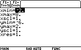
Press ◆◆ semicolon, then F2F2 to input window settings.
-
Press ◆◆ semicolon, then F3F3 to display the graph.